Effective 2D/3D Registration using Curvilinear Saliency Features and

Multi-Class SVM

Saddam Abdulwahab

, Hatem A. Rashwan

, Julian Cristiano

, Sylvie Chambon

and Domenec Puig

Department of Computer Engineering and Mathematics, Rovira i Virgili University, Tarragona, Spain

Department of Computing, IRIT, Universit

e de Toulouse, Toulouse, France

Keywords:

2D/3D Registration, Support Vector Machine, Cross Domain, Depth Images, Curvilinear Saliency.

Abstract:

Registering a single intensity image to a 3D geometric model represented by a set of depth images is still a

challenge. Since depth images represent only the shape of the objects, in turn, the intensity image is relative

to viewpoint, texture and lighting condition. Thus, it is essential to ﬁrstly bring 2D and 3D representations to

common features and then match them to ﬁnd the correct view. In this paper, we used the concept of curvilinear

saliency, related to curvature estimation, for extracting the shape information of both modalities. However,

matching the features extracted from an intensity image to thousand(s) of depth images rendered from a 3D

model is an exhausting process. Consequently, we propose to cluster the depth images into groups based on

Clustering Rule-based Algorithm (CRA). In order to reduce the matching space between the intensity and

depth images, a 2D/3D registration framework based on multi-class Support Vector Machine (SVM) is then

used. SVM predicts the closest class (i.e., a set of depth images) to the input image. Finally, the closest view

is reﬁned and veriﬁed by using RANSAC. The effectiveness of the proposed registration approach has been

evaluated by using the public PASCAL3D+ dataset. The obtaining results show that the proposed algorithm

provides a high precision with an average of 88%.

1 INTRODUCTION

Various object registration tasks and different compu-

ter vision applications such as human pose estimation,

face identiﬁcation and robotics use 2D intensity ima-

ges as input. Recently, 3D geometries are also availa-

ble and popular. Accordingly, taking the beneﬁt from

both modalities for 2D/3D matching has become ne-

cessary.

The 2D/3D registration is the problem of ﬁnding

the transformation and rotation of objects by mat-

ching their 3D models with 2D images. The matching

of a 2D image to a 3D model is considered a difﬁcult

task since the appearance of an object dramatically

depends on its intrinsic characteristics (e.g., texture

and color/albedo), and extrinsic characteristics rela-

ted to the acquisition (e.g., the camera pose and the

lighting conditions). The 2D/3D matching problem is

mainly about answering two main questions. (1) What

is the appropriate representation method that can be

used for extracting features in both 2D and 3D data?

(2) how to match entities between the two modalities

in this common representation?

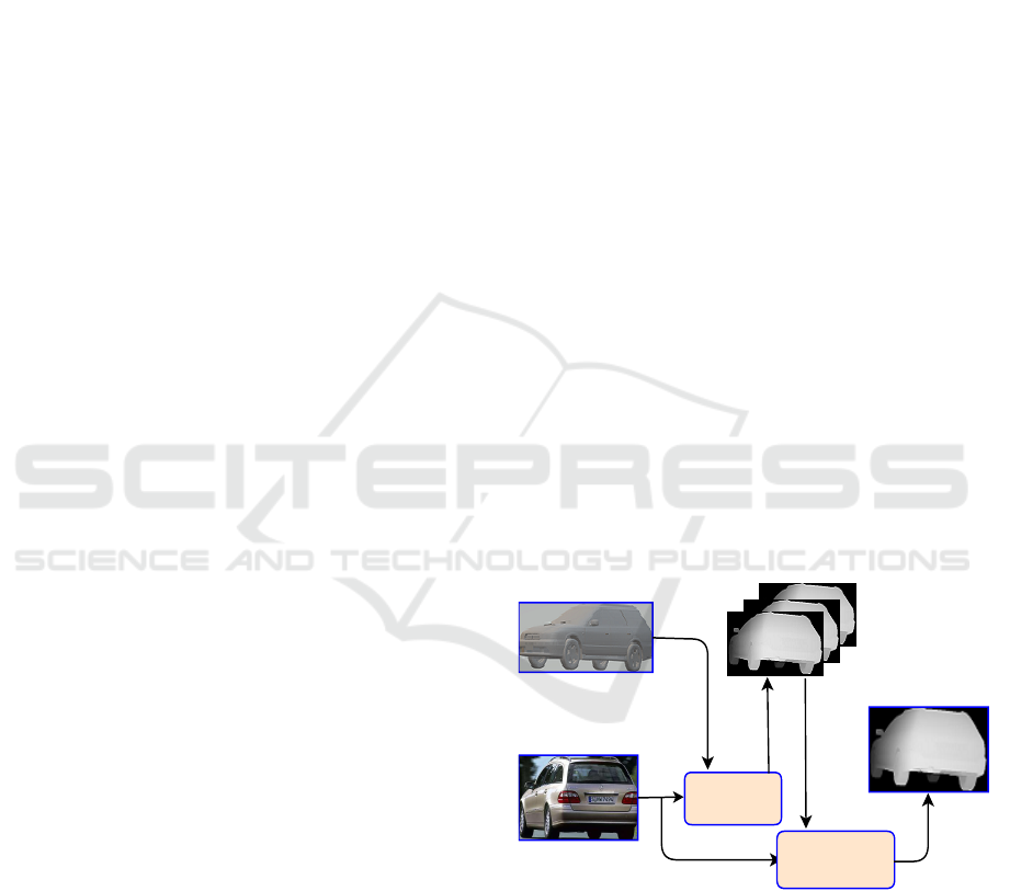
Many approaches have been proposed to extract

corresponding

depth image

SVM

Matching

(RANSAC)

3D model

Photograph

Cluster i

Prediction

Training

Test

Figure 1: General overview of the proposed 2D/3D regis-

tration algorithm.

features from 2D and 3D representation. For 3D mo-

dels, many possible ways are used to represent them.

To name few, synthetic images (Campbell and Flynn,

2001; Choy et al., 2015) of a 3D model were rende-

red. Silhouettes extracted from rendered images are

then matched to ones extracted from the intensity ima-

ges. However, these methods did not consider most

of the occluding contours that are useful for accurate

354

Abdulwahab, S., Rashwan, H., Cristiano, J., Chambon, S. and Puig, D.

Effective 2D/3D Registration using Curvilinear Saliency Features and Multi-Class SVM.

DOI: 10.5220/0007362603540361

In Proceedings of the 14th International Joint Conference on Computer Vision, Imaging and Computer Graphics Theory and Applications (VISIGRAPP 2019), pages 354-361

ISBN: 978-989-758-354-4

pose estimation. In addition, the silhouettes extrac-

ted from the image background can badly affect the

ﬁnal matching. More recently, (Pl

otz and Roth, 2017)

proposed average shading gradients (ASG), where the

gradient normals of all lighting directions were avera-

ged to cope with the unknown lighting of the query

image. The advantage of ASG is that it expresses the

3D model shape regardless of either colors or tex-

ture. Image gradients are then matched with ASG

images. However, image gradients are still affected

by image textures and background. Other works are

proposed in (Rashwan et al., 2016; Rashwan et al.,

2018). Where a collection of rendered images of the

3D models (i.e., depth images) from different view-

points were used to detect curvilinear features with

common basis deﬁnitions between depth and inten-

sity images. Furthermore, the authors in (Rashwan

et al., 2018) proposed three main steps. First, the rid-

ges and valleys of depth images rendered from the 3D

model were detected. In order to cope with the tex-

ture and background in 2D images, the features were

extracted by a multiscale scheme, and are then reﬁ-

ned by only keeping infocus features. The ﬁnal step

is to determine the correct 3D pose using a repeata-

ble K-NN registration algorithm (i.e., instance-based

learning) until ﬁnding the closest view. However, K-

NN algorithm is a simple machine learning algorithm

and a very exhausting process, as well as it is only

approximated locally.

Consequently, this work proposes an automatic

2D/3D registration approach reducing the matching

space and compensating the disadvantages of rende-

ring a large number of depth images. That is done

by clustering the features extracted from all rendered

images into N clusters using a Clustering Rule-based

Algorithm (CRA). The Histogram of Curviness Sa-

liency (HCS) is computed for each a depth image per

cluster. A multi-class SVM is then trained with the fe-

atures of each cluster for assigning a 2D real image to

the closest depth images. Finally, the closest view is

reﬁned by RANdom SAmple Consensus (RANSAC)

algorithm (Fischler and Bolles, 1987) by matching the

input image to the depth images belonging to the pre-

dicted class. Figure 1 shows the overview of the pro-

posed 2D/3D registration method.

In summary, the contributions of this paper are the

followings:

• updating a robust feature extraction method ba-

sed on curvilinear saliency proposed in (Rashwan

et al., 2018) for both 2D and 3D representations.

• clustering the features of the rendered depth ima-

ges of a 3D model into K clusters using CRA.

• cross-domain classiﬁcation based on a multi-class

SVM for assigning a query intensity image to a

class of the closest depth images.

• Determining the closest view using the RANSAC

algorithm.

The rest of the article is structured as follows:

Section 2 explains related works, and the proposed

methodology is detailed in Section 3. In addition, the

experiments and the results are shown in Section 4.

Finally, the conclusion and future work are discussed

in Section 5.

2 RELATED WORK

The problem of automatically aligning 2D intensity

images with a 3D model has been recently investi-

gated in depth. In the general case, the proposed

solution will be image-to-model registration to esti-

mate the 3D pose of the object. For various registra-

tion methods, the 3D models have been represented

in different ways (e.g., depth or synthetic images) and

then the features extracted from the query and rende-

red images are matched. In (Sattler et al., 2011; Lee

et al., 2013), correspondences were obtained by ma-

tching SIFT feature descriptors between SIFT points

extracted from the color images and from the 3D mo-

dels. However, establishing reliable correspondences

may be difﬁcult due to the fact that the features in 2D

and 3D are not always similar, in particular, because

of the variability of the illumination conditions during

the 2D and 3D acquisitions. Other methods relying on

higher level features, such as lines (Xu et al., 2017),

planes (Tamaazousti et al., 2011), building bounding

boxes (Liu and Stamos, 2005) and Skyline-based met-

hods (Ramalingam et al., 2009) have been generally

suitable for Manhattan World scenes and hence appli-

cable only in such environments.

Recently, the histogram of gradients, HOG, de-

tector (Aubry et al., 2014; Lim et al., 2014) or its

fast version proposed (Choy et al., 2015) have been

also used to extract the features from rendering views

and real images. These approaches have not evalua-

ted the repeatability between the correspondences de-

tected in an intensity image and those detected in ren-

dered images. In turn, 3D corner points have been

detected in (Pl

otz and Roth, 2017) using the 3D Har-

ris detector and the rendering ASG images have been

generated for each detected point. For a query image,

similarly, 2D corner pixels are detected in multiscale.

Then, the gradients computed for patches around each

pixel are matched with the database containing ASG

images using HOG descriptor. This method still re-

lies on extracting gradients of intensity images af-

fected by textures and background yielding erroneous

Effective 2D/3D Registration using Curvilinear Saliency Features and Multi-Class SVM

355

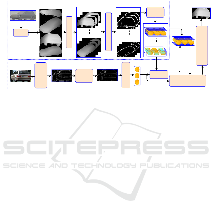
Rendering

Curviness Saliency Features

Detect Ridges using

Multi-scale

Curviness Saliency

Reﬁne by

detecting

Focus Curves

Dataset Depth

Images Rendering

3D model

Photograph

MCS image MFC image

Testing

Training

CRA

Cluster 1

Cluster N

Clustering images

Feature

Extraction

using HCS

SVM

images of Cluster i (RANSAC)

Cluster i

(N CS images)

Training

Prediction

viewpoint

(azimuth,elevation,distance)

Feature Extraction

using HCS

Vector

Cluster 1

Cluster N

Test

corresponding

depth image

Cluster 1

Cluster N

CS images

Figure 2: Registering a 2D image to a 3D model expressed by a collection of depth images rendered from different viewpoints,

and then extracting the curvilinear features of both depth and intensity images and after that, clustering the features of depth

images to k clusters using CRA. Training a multiclass SVM with the features of each cluster. Predicting the closest class to

the curvilinear features extracted with the query image. Finally, verifying the ﬁnal viewpoint using RANSAC.

correspondences. Finally, in (Rashwan et al., 2018),

the authors proposed structural cues (e.g., curvilinear

shapes) based on curvilinear saliency that are more ro-

bust to intensity, color, and pose variations, and both

outer and inner (self-occluding) contours are repre-

sented in these features. In order to merge in the

same descriptor curvilinear saliency values and curva-

ture orientation, the histogram of curvilinear saliency

(HCS) descriptor is proposed to properly describe the

object shape.

3 METHODOLOGY

This section explains the main steps of the proposed

scheme, the tools and the resources that have been

used in this work, in addition to the features used to

represent the 3D models and 2D images, and the ma-

chine learning method proposed. Figure 2 shows the

graphical description of the system. It contains two

main modules. The ﬁrst one is the SVM as a classi-

ﬁer, which is trained on a large set of features extrac-

ted from rendered depth images to assign a query 2D

image to a group of depth images. In subsection 3.3,

we explain in detail how we trained the SVM. The se-

cond module ﬁnds the closest rendered depth image

that matches a query 2D image to the predicted depth

images by using RANSAC in order to ﬁnd the ﬁnal

viewpoint. This module is described in subsection

3.4.

3.1 Labeling Depth Images based on

CRA

Unlike, the work proposed in (Su et al., 2015) by

rendering images of the 3D models based on varying

only the Azimuth angle, we represent every a 3D mo-

del by a set of depth images generated from various

camera locations distributed on concentric spheres en-

capsulating, by sampling elevation and azimuth an-

gles, as well as the distance from the camera to the

object. We rendered these depth images of 3D mo-

dels available in the online 3D model repository, PAS-

CAL3D+ (Xiang et al., 2014).

To reduce the space of matching between a single

intensity image and thousand(s) of depth images, the

rendered depth images are clustered to a set of groups.

Each cluster contains a group of depth images belon-

ging to a range of viewpoints. To assign each depth

image into a certain cluster, we deﬁned a set of rules

based on the azimuth and elevation angles, in addition

to the distance.

These rules are designed carefully to ensure that

all the samples in one category are inside a speciﬁc

range of viewpoints. Algorithm ?? shows the pro-

posed rules based on the maximum and minimum va-

lues of azimuth and elevation angles of rendering (i.e.,

max

, A

min

, E

max

and E

min

, respectively), in addition to

the the maximum and minimum values of the distance

of the camera to the 3D object (i.e., D

min

and D

max

In addition, Table 1 shows the clustering rules with

C = 9 used in this work.

VISAPP 2019 - 14th International Conference on Computer Vision Theory and Applications

356

Data: dataset

Result: K of clusters

Input: A

max

min

max

min

, D

max

min

Initialization:

a=(A

max

- A

min

) / C

e=(E

max

- E

min

) / C

while (i=1) <= C do

∈ [A

min

+ (i −1) ×a + 1, A

min

+ i ×a])

∈ [E

min

+ (i −1) ×e + 1, E

min

+ i ×e])

∈ [D

min

max

])

category=i

end

Algorithm 1: CRA used for clustering the depth images ba-

sed on (azimuth, elevation and distance) to G groups.

Table 1: CRA with C = 9 clusters of depth images consi-

dering A

max

= 180

and A

min

= 0

, E

max

= 90

and E

min

−90

, D

max

= 15 m and D

min

= 0.0 m.

Rule Category

∈ [0,20] ∧E

∈ [−90,−70]∧D

∈ [0,15]) 1

∈ [21,40] ∧E

∈ [−69,−50]∧D

∈ [0,15]) 2

∈ [41,60] ∧E

∈ [−49,−30]∧D

∈ [0,15]) 3

∈ [61,80] ∧E

∈ [−29,−10]∧D

∈ [0,15]) 4

∈ [81,100] ∧E

∈ [−9,10] ∧D

∈ [0,15]) 5

∈ [101,120] ∧E

∈ [11,30] ∧D

∈ [0,15]) 6

∈ [121,140] ∧E

∈ [31,50] ∧D

∈ [0,15]) 7

∈ [141,160] ∧E

∈ [51,70] ∧D

∈ [0,15]) 8

∈ [161,180] ∧E

∈ [71,90] ∧D

∈ [0,15]) 9

4 FEATURE EXTRACTION AND

DESCRIPTION

In order to obtain a common representation related to

the curvature estimation between the 3D model and

the 2D image to properly match them, this work uses

Curvilinear Saliency (CS) proposed (Rashwan et al.,

2018) to extract features of rendered depth images.

CS extracts saliency features in one scale and it can

be deﬁned as:

CS = 4

∇

(

−K) (1)

where ∇

∇

= [Z

]

is the ﬁrst derivative of a depth

image,

κ is the mean curvature and K its Gaussian

curvature.

In addition, to reduce the inﬂuence of the tex-

ture on the intensity images, we also use the curvili-

near saliency computation with a multi-scale scheme

(i.e., Multi-scale Curvilinear Saliency (MCS) pro-

posed in (Rashwan et al., 2018)) to extract scale-

invariant features of an intensity image. The curvi-

linear saliency of an intensity image at i scale can be

deﬁned as:

= α((I

+ I

)), (2)

where I

is the ﬁrst derivative of an intensity image

at scale i.

Furthermore, to reduce the effect of the back-

ground in color images, Multi-scale Focus Curves fe-

atures (MFC) proposed in (Rashwan et al., 2018) are

then used. MFC presents the focused features (i.e.,

curves) of a salient object in a scene and removes the

curves related to de-focused objects. The MFC featu-

res highlight salient features in intensity images that

are approximately similar to the detected features in

the depth images. This can be done by computing the

ratio between every two consecutive scales of the cur-

vilinear saliency scales R

as:

i+1

, (3)

given the maximum value R

in each scale level, the

blur amount s

at a scale can be calculated:

√

−1

, (4)

where σ

is the standard deviation of the re-blur Gaus-

sian at a scale. When a pixel of s

has a high value at

all scales, the maximum value of the blur amount s

used to build the ﬁnal MFC features:

MFC =

argmax

)

. (5)

To represent the curvilinear features extracted, the

Histogram of curvilinear saliency (HCS) is compu-

ted. HCS is similar to Histogram of Gradients (HOG),

which is robust to lighting changes and small variati-

ons in the pose. In HCS, the orientation of the curvi-

linear features (i.e., CS, MCS or MFC) in local cells

are binned into histograms for representing an image

or a sub-image. HCS has then been proved one of

the most beneﬁcial features in general object locali-

zation. In our experiments, we compute histograms

with 9 bins on cells of 5 ×5.

4.1 SVM Classiﬁer

The 2D/3D matching in this work will be achieved

as a multi-class supervised classiﬁcation problem ba-

sed on support vector machine (SVM). In particular,

a multi-class SVM is trained for features extracted of

depth images related to a cluster. A one-versus-all

training approach is applied. Thus, during the off-

line training stage, the SVM is trained with the fe-

ature vectors extracted from a set of depth images

that belong to a cluster. In turn, during the on-line

classiﬁcation stage, an input feature vector extracted

from a query intensity image is used for ﬁnding the

Effective 2D/3D Registration using Curvilinear Saliency Features and Multi-Class SVM

357

corresponding class with the largest output probabi-

lity following a winner-takes-all strategy. The ex-

perimental results conducted in this work have yiel-

ded the best classiﬁcation results by using non-linear

SVM with a kernel based on a Gaussian radial ba-

sis function (RBF) (γ = 0.2) and soft margin para-

meter (C = 1). In addition, the mapping kernel RBF

is deﬁned as: K(x

) = exp(−γkx

−x

), where

γ = 1/2σ

, kx

−x

is the squared Euclidean dis-

tance between the two feature vectors x

and x

, and σ

is a free parameter of the standard deviation.

Our classiﬁcation problem can be considered as a

cross-domain classiﬁcation. Since the training and the

validation, sets are related to a domain generated from

the features extracted from depth images, in turn, the

testing domain is the features extracted from 2D in-

tensity images.

The ﬁrst step to train a multi-class classiﬁer such

as SVM is to deﬁne a set of features from the in-

put images in dense real-valued vectors using the

HCS descriptor. As we explained in the afore-

mentioned subsection, we used the Curvilinear Sa-

liency Features (CS) (Rashwan et al., 2018) to ex-

tract the features of the training and the validation sets

(i.e., rendered depth images), in turn, the Multi-Scale

Curvilinear Saliency (MCS) or Multi-Focus Curves

(MFC) (Rashwan et al., 2018) are used to extract the

features of the testing set (intensity images). Once

we get all the samples for each cluster, the features of

each depth image are used for the SVM as a class to

train on. Then, the pre-trained model is used for the

on-line classiﬁcation of an intensity image to assign it

to a group of depth images.

4.2 Matching

In order to estimate the ﬁnal camera pose (i.e., azi-

muth, elevation and distance) of an input image rela-

tive to a 3D model, a 2D image will be matched to

depth images belonged to the predicted class provi-

ding from the SVM.

We sampled the curvilinear features of the input

image and all depth images related to the predicted

class to a set of key points. Matching between the

features represented by HCS for both real image and

depth images is then performed. RANSAC is ﬁnally

used to reﬁne the closest view and estimate the ﬁ-

nal pose. As proposed in (Plotz and Roth, 2015), in

each iteration of the inner RANSAC loop, we sam-

ple 6 correspondences to estimate both the extrinsic

and intrinsic parameters of the camera using the di-

rect linear transformation algorithm (Hartley and Zis-

serman, 2003). Few iterations of RANSAC (i.e., 20

iterations in this work) are sufﬁcient to ﬁnd a good re-

ﬁnement. The reﬁnement of coarse poses from a true

correspondence will usually converge to poses near

the ground truth.

5 EXPERIMENT AND RESULTS

This section describes the experiments performed to

evaluate the proposed model, in addition to the dataset

and the evaluation metrics used in the experiments.

Database

In this work, we used the PASCAL3D+ dataset (Xi-

ang et al., 2014), which contains 12 objects catego-

ries. Where every object contains around ten or more

3D models and more than 1000 real images related

to the category. All the real images are captured un-

der different conditions like lighting, complex back-

ground and low contrast. The depth images of the 3D

CAD models have been rendered using the viewpoint

information of the dataset. For all the tested 3D mo-

dels, we have rendered depth images using MATLAB

3D Model Renderer 7

from multi-viewpoint based

on changing azimuth and elevation angles, in addition

to the distance between the camera and the 3D model.

Results and Discussion

In all experiments, we tested the features extracted

from real images against the features extracted from

3D models. For each category of the PASCAL3D+

dataset, we computed the precision rate for detecting

the correct views after using the two aforementioned

methods for the 3D model representation, (i.e., CS,

and ASG), against the two techniques for the inten-

sity image representation (i.e., MCS and MFC). That

generates four variations of features used in the eva-

luation, such as MFC/CS, MCS/CS, MFC/ASG and

MCS/ASG. Some examples of the PASCAL3D+ da-

taset with CS, MCS and MFC features are shown in

ﬁgure 3.

Firstly, we tested the effect of dividing the image

(i.e., color or depth) into a number of cells with a spe-

ciﬁc size for describing an image on the accuracy of

the proposed 2D/3D registration. Thus, we computed

the precision rate of the registration process between

input intensity images and the rendered depth ima-

ges of each category of the PASCAL3D+ dataset with

different cell sizes, i.e., 3 ×3, 5 ×5 and 7 ×7 of the

HCS descriptor. Quantitative results with the average

precision rate over the 12 categories of PASCAL3D+

https://www.openu.ac.il/home/hassner/projects/poses/

VISAPP 2019 - 14th International Conference on Computer Vision Theory and Applications

358

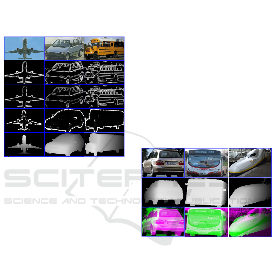
Table 2: Average Precision rates of the 5 categories of PASCAL3D+ with different cell sizes of the HCS descriptor.

Methods MFC/CS + SVM MCS/CS + SVM MFC/ASG + SVM MCS/ASG + SVM

HCS 3 × 3 0.65 0.53 0.56 0.53

HCS 5 × 5 0.88 0.84 0.84 0.79

HCS 7 × 7 0.77 0.73 0.72 0.66

Figure 3: intensity images (row 1), MCS resulting with 4

scales (row 2), MFC with 4 scales (row 3), CS (row 4)

and depth images (row 5). As it is shown, the curvilinear

saliency provided features closer to the features extracted

from depth images.

are shown in Table 2. As shown, the HCS with a cell

size 5 ×5 yielded the highest average precision with

the four variations of features. Therefore, we recom-

mended the HCS descriptor with a 5 ×5 cell size for

representing an image (depth or intensity).

Table 3 shows the effect of four different repre-

sentation of intensity images and 3D models (i.e.,

MFC/CS, MCS/CS, MFC/ASG and MCS/ASG) and

the classiﬁers (i.e., KNN and SVM), on the average

precision rate of the closest group. With all catego-

ries of PASCAL3D+, the performance of the propo-

sed model with SVM yielded better results than the

model with KNN. In addition For instance, with the

category of AEROPLANE and based on the represen-

tation of MFC/CS, the average precision rate with the

SVM was increased by 11% more than the KNN. In

turn, with TRAIN category, SVM yielded an impro-

vement of only 2%. The model with SVM as a classi-

ﬁer yielded an improvement in the average precision

rate of 6% with all categories of the PASCAL3D+.

For the features extracted from intensity images,

the image representation MFC with both representa-

tions of 3D models CS and ASG yielded a high pre-

cision rate comparing with the image representation

MCS. In addition, the 3D model representation CS

provided a higher precision rate than ASG. More pre-

cisely, MFC/CS with the SVM obtained an average

precision of around 88% with all categories of PAS-

CAL3D+. In addition, MFC/ASG with the SVM pro-

vided an average precision of about 83%. In turn,

MCS/CS with the SVM yielded an average precision

of around 83%, in turn, 80% with MCS/ASG. Accor-

ding to Table 3, the proposed model with MFC as an

intensity image representation, CS as a 3D model re-

presentation and SVM as a classiﬁer, performed better

regarding the average precision rate comparing with

the other variations models. We consider the above

results to be promising, as they are quite close to the

labelling of PASCAL3D+. Three examples of the ﬁ-

nal registration based on MFC/CS and with SVM are

shown in Figure 4.

Figure 4: Three examples of the proposed 2D/3D regis-

tration model with the Pascal3D+ dataset, query intensity

images (row 1), the resulted ﬁnal depth images (row 2) and

the composite image from the intensity and resulted depth

image (row 3). As shown even if the 3D model does not

have the same detailed shape, the registration can properly

be achieved.

For viewpoint evaluation, we compare with three

methods using the same dataset, PASCAL3D+. A re-

cent work has been proposed in (Tulsiani and Ma-

lik, 2015), which introduced to a CNN architecture

to predict viewpoint, and combines multiscale ap-

pearance with a viewpoint conditioned likelihood to

predict key-points to capture the ﬁner details to cor-

rectly detect the bound-box of the objects. In addi-

tion, our model was compared with the work propo-

sed in (Szeto and Corso, 2017), which presented a

deep model based on CNN for monocular viewpoint

estimation by using key points information provided

Effective 2D/3D Registration using Curvilinear Saliency Features and Multi-Class SVM

359

Table 3: Precision of pose estimation CS, ASG against MFC, MCS using SVM and KNN.

MFC/CS MCS/CS MFC/ASG MCS/ASG

Methods

SVM KNN SVM KNN SVM KNN SVM KNN

aere 0.93 0.85 0.85 0.83 0.91 0.84 0.81 0.80

bus 0.92 0.87 0.84 0.82 0.83 0.82 0.80 0.80

car 0.92 0.86 0.87 0.85 0.89 0.86 0.85 0.83

sofa 0.75 0.85 0.73 0.81 0.68 0.81 0.72 0.72

train 0.88 0.87 0.87 0.86 0.85 0.81 0.82 0.82

mean 0.88 0.86 0.83 0.83 0.83 0.83 0.80 0.79

Table 4: Viewpoint estimation with ground truth bounding box. Evaluation metrics are deﬁned in (Tulsiani and Malik, 2015),

where Acc

π/6

measures accuracy (the higher the better). N/A means that the tested work did not show the results with these

categories.

aera bus car sofa train mean

Acc

π/6

(Su et al., 2015) 0.74 0.91 0.88 0.90 0.86 0.86

Acc

π/6

(Tulsiani and Malik, 2015) 0.81 0.98 0.89 0.82 0.80 0.86

Acc

π/6

( (Szeto and Corso, 2017) KPC Only) N/A 0.91 0.86 N/A N/A 0.89

Acc

π/6

( (Szeto and Corso, 2017) KPM Only) N/A 0.91 0.82 N/A N/A 0.87

Acc

π/6

( (Szeto and Corso, 2017) Full Model) N/A 0.97 0.90 N/A N/A 0.94

Acc

π/6

(Our Model) 0.93 0.92 0.92 0.75 0.88 0.88

by humans at inference time to more accurately es-

timate the viewpoint of an object. Furthermore, we

compared our model to the work introduced in (Su

et al., 2015) that rendered millions of synthetic ima-

ges from 3D models under varying illumination, lig-

hting and backgrounds and then used them to train a

CNN model for viewpoint estimation of real images.

We used the same metrics Acc

π/6

as in (Tulsiani and

Malik, 2015), for more details of the metric deﬁnition,

please refer to (Tulsiani and Malik, 2015). Quanti-

tative results are shown in Table 4. As shown, we

shows the ﬁnal results of ﬁner viewpoint estimation

that used the SVM classiﬁer with HCS and RANSAC

to reﬁne the ﬁnal 3D pose. Our model yielded the

best average accuracy among all tested methods with

88%. The works proposed in (Su et al., 2015; Tulsiani

and Malik, 2015) yielded an acceptable accuracy of

86%. These methods have rendered millions of synt-

hetic images to train their deep models. Note that the

authors of (Szeto and Corso, 2017) have shown only

the results of two categories, thus the average accu-

racy was computed for just these two categories. The

proposed model achieved a high accuracy with the

AEROPLANE and CAR categories, since MFC can

provide adequate shape features for these types of ob-

jects. Moreover, real images used in testing always

contain simple backgrounds. However, the SOFA ca-

tegory did not provide a high accuray, since the most

of 3D model of SOFA have a similar shape. In ad-

dition, real images have more complex backgrounds

than other categories.

The proposed model was implemented using

MATLAB on a 64-bit CPU with 3.40 GHz, 16 GB

memory, and NVIDIA GTX 1070 GPU. In ﬁgure 5,

the complexity of the computational time of each task

of the proposed method, i.e., rendering, depth feature

extraction, training SVM, image feature extraction

(MFC, MCS, CS), on-line SVM prediction and RAN-

SAC, is shown as a Pie chart. As shown, the most exe-

cution time that is about 76% of the total time is rela-

ted to off-line tasks, such as rendering, depth features

extraction and training SVM. In turn, to predict the

ﬁnal viewpoint that means the online prediction, the

other three tasks (i.e., feature extraction of an image,

on-line SVM prediction and RANSAC) take around

24% of the total computational time.

Figure 5: The percentage of the time consuming with each

subsystem of the proposed approach.

6 CONCLUSIONS

In this work, we have proposed an automatic 2D/3D

registration approach compensating the disadvantages

of rendering a large number of images of 3D models

VISAPP 2019 - 14th International Conference on Computer Vision Theory and Applications

360

(i.e., depth images) by reducing the matching space

between the 2D intensity and 3D depth images. The

depth images rendered of a 3D model were represen-

ted with the curvilinear saliency features. In addition,

an accurate representation based on multi-scale curvi-

linear saliency with focus features was used to reduce

the effect of texture and background on the extrac-

ted features of an intensity image. The depth ima-

ges were clustered with a rule-based clustering met-

hod. The features of each cluster of depth images

were used to train a multi-class SVM for estimating

a group of depth images that are close to the input in-

tensity image. The matching between the input image

and the predicted class was then performed to esti-

mate the correct 3D pose. The RANSAC algorithm

was used to reﬁne and verify the ﬁnal viewpoint. The

effectiveness of the proposed system has been evalu-

ated on the public PASCAL3D+ dataset. The propo-

sed 2D/3D registration algorithm yielded promising

results with a high precision rate and acceptable com-

putational timing. Future work aims to extend the pre-

sented 2D/3D registration algorithm using a deep le-

arning system.

REFERENCES

Aubry, M., Maturana, D., Efros, A. A., Russell, B. C., and

Sivic, J. (2014). Seeing 3d chairs: exemplar part-

based 2d-3d alignment using a large dataset of cad

models. In Proceedings of the IEEE conference on

computer vision and pattern recognition, pages 3762–

3769.

Campbell, R. J. and Flynn, P. J. (2001). A survey of free-

form object representation and recognition techni-

ques. Computer Vision and Image Understanding,

81(2):166–210.

Choy, C. B., Stark, M., Corbett-Davies, S., and Savarese, S.

(2015). Enriching object detection with 2d-3d regis-

tration and continuous viewpoint estimation. In Com-

puter Vision and Pattern Recognition (CVPR), 2015

IEEE Conference on, pages 2512–2520. IEEE.

Fischler, M. A. and Bolles, R. C. (1987). Random sample

consensus: a paradigm for model ﬁtting with appli-

cations to image analysis and automated cartography.

In Readings in computer vision, pages 726–740. Else-

vier.

Hartley, R. and Zisserman, A. (2003). Multiple view geome-

try in computer vision. Cambridge university press.

Lee, Y. Y., Park, M. K., Yoo, J. D., and Lee, K. H. (2013).

Multi-scale feature matching between 2d image and

3d model. In SIGGRAPH Asia 2013 Posters, page 14.

ACM.

Lim, J. J., Khosla, A., and Torralba, A. (2014). Fpm: Fine

pose parts-based model with 3d cad models. In Euro-

pean Conference on Computer Vision, pages 478–493.

Springer.

Liu, L. and Stamos, I. (2005). Automatic 3d to 2d registra-

tion for the photorealistic rendering of urban scenes.

In Computer Vision and Pattern Recognition, 2005.

CVPR 2005. IEEE Computer Society Conference on,

volume 2, pages 137–143. IEEE.

Plotz, T. and Roth, S. (2015). Registering images to untex-

tured geometry using average shading gradients. In

Proceedings of the IEEE International Conference on

Computer Vision, pages 2030–2038.

otz, T. and Roth, S. (2017). Automatic registration of

images to untextured geometry using average shading

gradients. International Journal of Computer Vision,

125(1-3):65–81.

Ramalingam, S., Bouaziz, S., Sturm, P., and Brand, M.

(2009). Geolocalization using skylines from omni-

images. In Computer Vision Workshops (ICCV Works-

hops), 2009 IEEE 12th International Conference on,

pages 23–30. IEEE.

Rashwan, H. A., Chambon, S., Gurdjos, P., Morin, G., and

Charvillat, V. (2016). Towards multi-scale feature

detection repeatable over intensity and depth images.

In Image Processing (ICIP), 2016 IEEE International

Conference on, pages 36–40. IEEE.

Rashwan, H. A., Chambon, S., Gurdjos, P., Morin, G., and

Charvillat, V. (2018). Using curvilinear features in fo-

cus for registering a single image to a 3d object. arXiv

preprint arXiv:1802.09384.

Sattler, T., Leibe, B., and Kobbelt, L. (2011). Fast image-

based localization using direct 2d-to-3d matching. In

Computer Vision (ICCV), 2011 IEEE International

Conference on, pages 667–674. IEEE.

Su, H., Qi, C. R., Li, Y., and Guibas, L. J. (2015). Render for

cnn: Viewpoint estimation in images using cnns trai-

ned with rendered 3d model views. In Proceedings of

the IEEE International Conference on Computer Vi-

sion, pages 2686–2694.

Szeto, R. and Corso, J. J. (2017). Click here: Human-

localized keypoints as guidance for viewpoint estima-

tion. arXiv preprint arXiv:1703.09859.

Tamaazousti, M., Gay-Bellile, V., Collette, S. N., Bour-

geois, S., and Dhome, M. (2011). Nonlinear reﬁne-

ment of structure from motion reconstruction by ta-

king advantage of a partial knowledge of the envi-

ronment. In Computer Vision and Pattern Recogni-

tion (CVPR), 2011 IEEE Conference on, pages 3073–

3080. IEEE.

Tulsiani, S. and Malik, J. (2015). Viewpoints and keypoints.

In Proceedings of the IEEE Conference on Computer

Vision and Pattern Recognition, pages 1510–1519.

Xiang, Y., Mottaghi, R., and Savarese, S. (2014). Beyond

pascal: A benchmark for 3d object detection in the

wild. In Applications of Computer Vision (WACV),

2014 IEEE Winter Conference on, pages 75–82. IEEE.

Xu, C., Zhang, L., Cheng, L., and Koch, R. (2017). Pose

estimation from line correspondences: A complete

analysis and a series of solutions. IEEE transacti-

ons on pattern analysis and machine intelligence,

39(6):1209–1222.

Effective 2D/3D Registration using Curvilinear Saliency Features and Multi-Class SVM

361