Pedestrian Intensive Scanning for Active-scan LIDAR

Taiki Yamamoto

, Fumito Shinmura

, Daisuke Deguchi

Yasutomo Kawanishi

, Ichiro Ide

and Hiroshi Murase

Graduate School of Informatics, Nagoya University, Furo-cho, Chikusa-ku, Nagoya-shi, Aichi, Japan

Institutes of Innovation for Future Society, Nagoya University, Furo-cho, Chikusa-ku, Nagoya-shi, Aichi, Japan

Information Strategy Ofﬁce, Nagoya University, Furo-cho, Chikusa-ku, Nagoya-shi, Aichi, Japan

Keywords:

Active-scan LIDAR, Stochastic Sampling, Pedestrian Detection.

Abstract:

In recent years, LIDAR is playing an important role as a sensor for understanding environments of a vehicle’s

surroundings. Active-scan LIDAR is being actively developed as a LIDAR that can control the laser irradiation

direction arbitrary and rapidly. In comparison with conventional uniform-scan LIDAR (e.g. Velodyne HDL-

64e), Active-scan LIDAR enables us to densely scan even distant pedestrians. In addition, if appropriately

controlled, this sensor has a potential to reduce unnecessary laser irradiations towards non-target objects.

Although there are some preliminary studies on pedestrian scanning strategy for Active-scan LIDARs, in the

best of our knowledge, an efﬁcient method has not been realized yet. Therefore, this paper proposes a novel

pedestrian scanning method based on orientation aware pedestrian likelihood estimation using the orientation-

wise pedestrian’s shape models with local distribution of measured points. To evaluate the effectiveness of the

proposed method, we conducted experiments by simulating Active-scan LIDAR using point-clouds from the

KITTI dataset. Experimental results showed that the proposed method outperforms the conventional methods.

1 INTRODUCTION

In recent years, development of autonomous driving

systems and Advanced Driver Assistance Systems

(ADAS) is attracting attention all over the world. Col-

lision avoidance is one of the most important function

in these systems to reduce trafﬁc accidents, and re-

cognition of surrounding environments is indispensa-

ble for developing these systems. Currently, various

types of sensors have been developed and some of

them are commercially available. Among them, LI-

DAR (LIght Detection And Ranging) is now widely

implemented as an in-vehicle sensor for recognizing

the surrounding environment. LIDAR can simultane-

ously measure the distance to target objects and their

reﬂection intensities by irradiating laser rays and me-

asuring their reﬂections. Velodyne LiDAR

is one of

the most popular LIDAR in recent years, which is

equipped with multiple laser irradiation ports in the

vertical direction as shown in Fig. 1. Irradiating la-

ser rays by rotating the sensor itself in the horizon-

tal direction, it can obtain a point-cloud of 360 de-

grees view uniformly (We call this type of LIDAR as

Velodyne LiDAR, Inc. https://velodynelidar.com/

“uniform-scan LIDAR”). In addition, according to the

increase of laser irradiation ports, the vertical density

of the point-cloud can be increased.

Some research groups tackled the problem

of pedestrian detection devising uniform-scan LI-

DARs (Kidono et al., 2011; Behley et al., 2013; Ma-

turana and Scherer, 2015; Wang et al., 2017; Tatebe

et al., 2018; Zhou and Oncel, 2018). Kidono et al.

proposed two kinds of features for recognizing pede-

strians using a dense uniform-scan LIDAR (Kidono

et al., 2011). Their method extracts a slice feature

which is deﬁned by the horizontal and depth sizes of

3D point-clouds in each vertically sliced section for a

rough shape representation. In addition, they propo-

sed an additional feature which is the reﬂection inten-

sity distribution for representing the material of the

target surface. Based on these features, it is possible

to distinguish pedestrians with non-pedestrians such

as poles. Although their method succeeded to detect

most pedestrians, its accuracy degraded if the target

pedestrian exists in a distant position.

To cope with this problem, Tatebe et al. pro-

posed a voxel representation method applicable to

sparse point-clouds that are obtained from distant tar-

gets (Tatebe et al., 2018). Their method combined

Yamamoto, T., Shinmura, F., Deguchi, D., Kawanishi, Y., Ide, I. and Murase, H.

Pedestrian Intensive Scanning for Active-scan LIDAR.

DOI: 10.5220/0007359903130320

In Proceedings of the 14th International Joint Conference on Computer Vision, Imaging and Computer Graphics Theory and Applications (VISIGRAPP 2019), pages 313-320

ISBN: 978-989-758-354-4

313

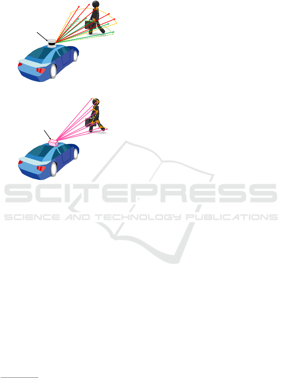
LIDAR

Figure 1: Scanning using a LIDAR.

Active Scan

LIDAR

Figure 2: Scanning using an Active Scan LIDAR.

the voxel representation and 3DCNN for pedestrian

detection. By using the characteristic that the beam

width of an irradiated laser ray increases according to

the distance from the sensor, their method estimates

the distribution of the target point-cloud and uses it for

constructing a voxel representation. Although they

succeeded to detect distant pedestrians, their method

still failed if the density of the target point-cloud is

extremely low. Therefore, improvement of the point-

cloud density will be the key factor to improve the

detection accuracy of distant pedestrians. However, it

is difﬁcult for an uniform-scan LIDAR to increase the

vertical density of the point-cloud because the number

of laser irradiation ports is limited.

Recently, some manufacturers are trying to deve-

lop new types of LIDARs that can control the laser

irradiation direction arbitrary and rapidly as shown

in Fig. 2, such as Blackmore Sensors and Analytics,

Inc

. Hereafter, we call these types of sensors as

Active-scan LIDAR. It has a great advantage which

enables us to scan arbitral 3D positions quickly and

programmatically. If we can control it appropriately,

we can expect to obtain a dense point-cloud of dis-

tant pedestrians as same as close pedestrians. Since

Blackmore Sensors and Analytics, Inc. https://

blackmoreinc.com/

scanning time increases according to the number of

irradiated laser rays, it is necessary to properly set la-

ser irradiation directions to obtain a dense point-cloud

of pedestrians efﬁciently.

To solve this problem, we proposed a progres-

sive scan strategy using pedestrian’s shape model to

obtain dense point-clouds from pedestrians (Yama-

moto et al., 2018). Although the observable pede-

strian’s shape changes according to the viewpoint (or

pedestrian’s orientation), the method did not consider

the variations of observable shapes. In addition, since

the method constructed a pedestrian likelihood map

by assuming that all measured points came from pe-

destrians, we did not segregate the measured points

from non-pedestrian objects. Thus, it was difﬁcult to

distinguish a point-cloud of a pedestrian from that of

a non-pedestrian object, such as a pole or a tree that

has a similar shape as a pedestrian but has a different

size.

To overcome the above problems, this paper pro-

poses an orientation-aware pedestrian scanning met-

hod that enables us to scan pedestrians densely with

a small number of laser irradiations. In the propo-

sed method, the pedestrian’s orientation is considered

when constructing his/her shape model. Moreover,

a pedestrian likelihood map is calculated by conside-

ring whether the measured points came from the same

object or not. Here, depth-wise object separation is

used. Finally, we formulate the selection of laser ir-

radiation directions as a problem in a stochastic sam-

pling framework based on the pedestrian likelihood

map.

The contributions of this paper are as follows:

1. Estimation of a pedestrian likelihood map consi-

dering observable pedestrian’s shape variation ac-

cording to his/her orientation.

2. Introduction of depth-wise object separation for

constructing the pedestrian likelihood map con-

sidering whether the measured points came from

the same object or not.

2 IDEAS FOR EFFICIENT

SCANNING

This section describes the basic ideas to efﬁciently

obtain a dense point-cloud from a pedestrian efﬁ-

ciently devising an Active-scan LIDAR. In order to

select appropriate laser irradiation directions, the pro-

posed method employs a stochastic sampling frame-

work based on a pedestrian likelihood map represen-

ting the existence of pedestrians. Here, the primary

pedestrian likelihood map is constructed by the initial

VISAPP 2019 - 14th International Conference on Computer Vision Theory and Applications

314

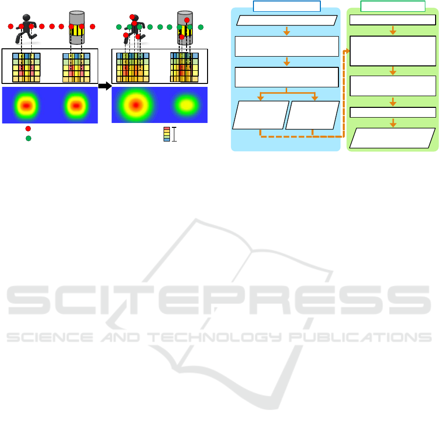
Initial scan

Adaptive scan

Additional points

Previous points

High

Low

Likelihood

Figure 3: Increasing the number of measured points and

updating the pedestrian likelihood map by adaptive scan.

scan, and then the proposed method progressively up-

dates the pedestrian likelihood map based on the me-

asured points by additional laser irradiations where

their directions are set adaptively. By repeating this

step, the pedestrian likelihood map gradually impro-

ves even if the initial point-cloud is sparse, as shown

in Fig. 3.

Here, considering the observable shape variati-

ons among front, back, right, and left orientations,

multiple pedestrian’s shape models are integrated to

compute the pedestrian likelihood map. Futhermore,

the pedestrian likelihood map is calculated by con-

sidering whether the measured points came from the

same object or not. Here, depth-wise object separa-

tion based on the pedestrian’s shape model is applied

to judge whether the points are measured within the

same object or not. Then, the proposed method calcu-

lates the ratio of pedestrian/non-pedestrian points ba-

sed on the above, and uses it for controlling the weig-

hts representing the goodness of ﬁtted pedestrian’s

shape model. Finally, the selection of the next laser

irradiation directions are stochastically sampled from

the pedestrian likelihood map.

Here, the pedestrian likelihood map M

(x, y) in the

t-th iteration is calculated as

(x, y) =

∑

p∈P

∑

F(x, y | p

p,θ), (1)

where P

is a point-cloud obtained until the t-th scan,

θ is a parameter corresponding to the orientation of

the pedestrian’s model, and F(x, y | p

p,θ) is a local pe-

destrian likelihood map when a point p

p and θ are gi-

ven. The local pedestrian likelihood map F(x, y | p

p,θ)

is calculated as

F(x, y | p

p,θ) = G(p

p | θ)H(p

p | θ)S(x,y | p

p,θ), (2)

where G(p

p | θ) represents the goodness of the ﬁtted

pedestrian’s shape model around the given p

p, H(p

p | θ)

Training phase

Pedestrians’ point-clouds

Scanning phase

Generation of depth map and

pedestrian shape prior map

Initial scan

Calculation of

, ,

and AAAAAA

Generation of pedestrian

likelihood map AAA

Adaptive scan

Point-cloud of

scanning result

Depth map

(4 orientations)

Pedestrian

shape prior map

(4 orientations)

Preparation of pedestrians’

point-clouds for each orientation

G(p

p | θ)

H(p

p | θ)

S(x, y | p

p, θ)

(x, y)

Figure 4: Process-ﬂow of the proposed method.

represents the degree of object isolation around p

p, and

S(x, y | p

p,θ) is the local probability map representing

pedestrian existence around p

Based on the stochastic sampling from the pede-

strian likelihood map M

(x, y), the directions of the la-

ser irradiations for the (t + 1)-th scan are calculated.

After completing the (t + 1)-th scan, the (t + 1)-th pe-

destrian likelihood map M

t+1

(x, y) is calculated.

3 ADAPTIVE SCANNING BASED

ON PEDESTRIAN

LIKELIHOOD

This section describes the proposed method to realize

the ideas explained in Section 2. Figure 4 shows the

process-ﬂow of the proposed method. It consists of

the following two phases:

1. Training phase

(a) Preparation of pedestrians’ point-clouds for

each orientation

(b) Generation of depth maps and pedestrian shape

prior maps

2. Scanning phase

(a) Initial scan

(b) Calculation of G(p

p | θ), H(p

p | θ), and S(x,y |

p,θ) using depth maps and pedestrian shape

prior maps

(x, y)

(d) Adaptive scan based on pedestrian likelihood

map M

(x, y)

(e) Repeat 2(b) to 2(e)

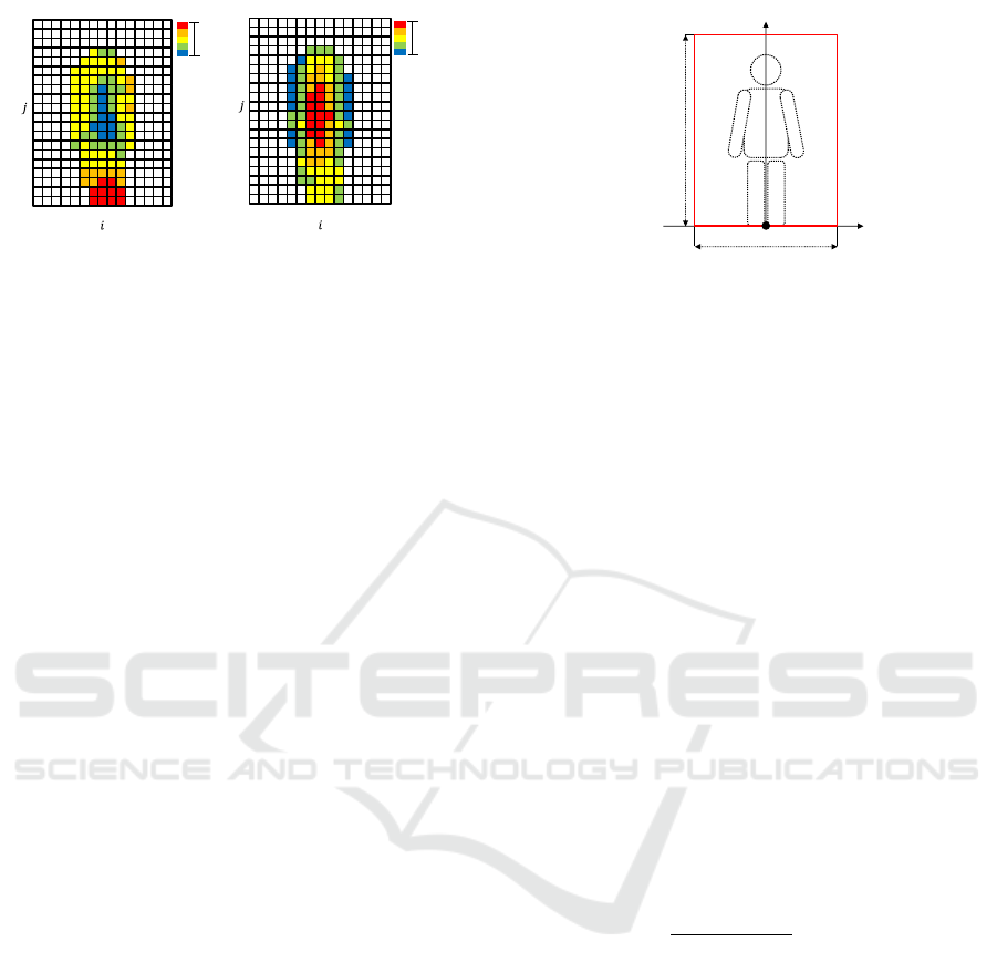
In the training phase, depth maps and pedestrian

shape prior maps are constructed from manually ex-

Pedestrian Intensive Scanning for Active-scan LIDAR

315

far

near

Average depth

-7

1-1

⋯

(a) Depth map.

high

low

Value

-7

1-1

⋯

(b) Pedestrian shape prior

map.

Figure 5: Example of a depth map and a pedestrian shape

prior map for the front orientation.

tracted pedestrians’ point-clouds, and their orienta-

tions are also manually annotated. In the scanning

phase, laser irradiation directions are adaptively se-

lected based on a stochastic sampling from the pe-

destrian likelihood map M

(x, y), and those measure-

ment results are used for updating the pedestrian li-

kelihood map M

t+1

(x, y) for the next scan. Details of

each process are described below.

3.1 Training Phase

This section describes the generation of two maps that

represent depth and pedestrian shape prior for each

orientation of pedestrians. The depth maps are used

for calculating G(p

p | θ) and H(p

p | θ) and the pede-

strian shape prior maps are used to calculate S(x , y |

p,θ) in Eq. (2). In the following explanation, for sim-

plicity, the position of LIDAR is set at the origin of the

coordinate system, and x-, y-, and z-axes of the coor-

dinate system correspond to the lateral, the vertical,

and the depth directions of the vehicle, respectively.

3.1.1 Preparation of Pedestrians’ Point-clouds

for Each Orientation

First of all, pedestrians’ point-clouds are extracted

from LIDAR data, and then they are classiﬁed into

four pedestrian’s orientation (front, back, left, right)

manually. Here, pedestrians’ point-clouds difﬁcult to

be classiﬁed into any of the four orientations are dis-

carded.

3.1.2 Calculation of Depth Maps and Pedestrian

Shape Prior Maps

The depth maps and the pedestrian shape priors are

calculated by integrating pedestrians’ point-clouds in

each orientation. Figure 5 shows an example of a

depth map and a pedestrian shape prior map for the

front orientation.

1.5 m

2.0 m

Figure 6: Points are extracted from an area with a size of

1.5 m × 2.0 m.

The ﬁrst step is the integration of pedestrians’

point-clouds in each orientation. Here, point-clouds

are aligned by shifting each point-cloud so that the

smallest vertical coordinate (y-axis), depth coordi-

nate (z-axis), and the average of the lateral coordi-

nate (x-axis) become zero. After the alignment, as

shown in Fig. 6, points are extracted from an area

with a size of 1.5 m × 2.0 m. Finally, the integra-

ted point-clouds are divided into 15 × 20 cells and

are used for calculating the depth map and the pe-

destrian shape prior map. Here, each cell has a size

of W × W (W = 0.1 m), and is identiﬁed using hori-

zontal and vertical indices (i = −7,−6,...,0,...,6, 7,

j = 0, 1, ..., 19).

From the integrated point-clouds, the depth map

of each orientation d(i, j | θ) is calculated as the

average depth in each cell where θ is a parameter

indicating the orientation of the pedestrian’s model.

Also, the pedestrian shape prior map of each orien-

tation s(i, j | θ) is calculated based on the number of

points n(i, j | θ) contained in each cell as

s(i, j | θ) =











n(i, j | θ)

∑

k,ℓ

n(k, ℓ | θ)

if n(i, j | θ) ≥ 10

and |i| ≤ 7

and 0 ≤ j ≤ 19

0 otherwise

(3)

Here, to reduce the effect of noise, if the cell satisﬁes

n(i, j | θ) < 10, they are treated as d(i, j | θ) = ∞ and

n(i, j | θ) = 0. Finally, d(i, j | θ) and s(i, j | θ) are

used as a depth map and a pedestrian shape prior map,

respectively.

3.2 Scanning Phase

This section describes the adaptive selection of laser

irradiation directions based on a stochastic sampling

from the pedestrian likelihood map. Details on the

calculation process of the pedestrian likelihood map

is also described.

VISAPP 2019 - 14th International Conference on Computer Vision Theory and Applications

316

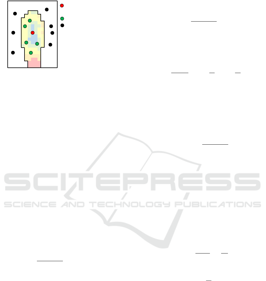
Point to calculate

the pedestrian likelihood

Neighbors of

Surrounding points of

p | θ)

(

)

Figure 7: Points used for calculating the weights G(p

p | θ)

and H(p

p | θ).

3.2.1 Initial Scan

As the ﬁrst step, the initial scan is performed to ﬁnd a

pedestrian by a small number of laser irradiations to

obtain the rough shape and position of each object in a

scene. Here, the initial number of laser irradiations is

, and each laser ray is irradiated at a certain interval

along the horizontal direction at a constant height h.

After the initial scan, a horizontally dense point-cloud

at the height h is obtained.

3.2.2 Calculation of Weights and the Local

Probability Map using Depth Maps and

Pedestrian Shape Prior Maps

As the second step, the global pedestrian likelihood

map (Eq. (2)) is calculated by G(p

p | θ), H(p

p | θ), and

S(x, y | p

p,θ) where S(x, y | p

p,θ) is the local probability

map around p

p, and G(p

p | θ) and H(p

p | θ) are weights

for controlling the integration of S(x, y | p

p,θ).

First of all, based on a point p

p ∈ P

obtained after

the t-th scan, G(p

p | θ) representing the goodness of

the ﬁtted pedestrian’s shape is calculated as

G(p

p | θ) =

p | θ)|

∑

q∈N

p|θ)

ϕ(p

p,q

q | θ), (4)

where N

p | θ) is a set of neighbor points coming

from the same object around p

p and |N

p | θ)| is the

number of points in N

p | θ). N

p | θ) is obtained

p | θ) = {q

q | q

q ∈ P

,ϕ(p

p,q

q | θ) ̸= 0,

− p

| ≤ 0.75 m,0 m ≤ q

≤ 2 m,

− p

| ≤ 1 m},

(5)

where p

p = (p

, p

) and q

q = (q

). An ex-

ample of neighbor points of a pedestrian around p

(red point) is shown in Fig. 7 (green points). Here,

ϕ(p

p,q

q | θ) is a normal distribution whose average and

variance are µ = d(i, j | θ) − d(0,c | θ) and σ

, re-

spectively, and is calculated as

ϕ(p

p,q

q | θ) =



exp



−

((q

−p

)−µ)

2σ



if d(i, j | θ) ̸= ∞

0 otherwise

(6)

where d(0,c | θ) is the depth of the cell (0, c) con-

taining p

p, and d(i, j | θ) is the depth of the cell (i, j)

containing q

q. The indices i, j, and c are calculated as

i =



− p



, j =





,c =





. (7)

Note that ⌊·⌋ is a ﬂoor function deﬁned as

⌊x⌋ = max{n | ∀n ∈ I, n ≤ x}, (8)

where I is a set of whole integers.

H(p

p | θ) corresponds to the weight for controlling

the effect of G(p

p | θ) based on depth-wise object se-

paration around p

p, which is calculated as

H(p

p | θ) =

p | θ)|

, (9)

where N

p | θ) is a set of surrounding points co-

ming from different objects around p

p (black points)

and |N

p | θ)| is the number of points in N

p | θ).

Here, N

p | θ) is obtained as

p | θ) = {q

q | q

q ∈ P

,ϕ(p

p,q

q | θ) = 0,

− p

| ≤ 0.75 m,0 m ≤ q

≤ 2 m,

− p

| ≤ 1 m}.

(10)

S(x, y | p

p,θ) is the local probability map represen-

ting the existence of a pedestrian around p

p, which is

calculated as

S(x, y | p

p,θ) = s



x − p

′





′







, (11)

where W

′

is calculated as

′

. (12)

3.2.3 Calculation of Pedestrian Likelihood Map

As the third step, the pedestrian likelihood map

(x, y) is generated using the weights G(p

p | θ) and

H(p

p | θ) and the local probability map S(x, y | p

p,θ)

derived in Section 3.2.2.

The pedestrian likelihood map M

(x, y) is calcula-

ted by Eqs. (1) and (2).

Pedestrian Intensive Scanning for Active-scan LIDAR

317

3.2.4 Adaptive Scan based on the Pedestrian

Likelihood Map

Finally, the laser irradiation directions are selected for

the next scan. The stochastic sampling referring to the

probability of the existence of pedestrians represented

by the pedestrian likelihood map M

(x, y) is applied to

select irradiation directions. Here, the inverse trans-

form sampling (Devroye, 1986) is used as the stochas-

tic sampling. Then, ∆N laser rays are irradiated in the

(t + 1)-th scan.

4 EXPERIMENTS

We conducted the experiment for evaluating the pe-

formance of the proposed method. The following

sections explain details of the experimental settings

and discuss the results.

4.1 Datasets

Since the hardware of an Active-scan LIDAR that can

control the laser irradiation direction arbitrary and ra-

pidly is still under development, we cannot use it for

our experiments. Therefore, here we mimic the beha-

vior of an Active-scan LIDAR by using dense point-

clouds that are obtained by a higher density uniform

scan LIDAR. For training, 400 point-clouds of pede-

strians were collected (100 point-clouds for each pe-

destrian’s orientation). Here, Velodyne LiDAR HDL-

64E was used for obtaining point-clouds in a real-

world environment, and these training data were used

for generating the depth map and the local pedestrian

likelihood map. On the other hand, for testing, we

used the KITTI dataset (Geiger et al., 2012) and the

Active-scan LIDAR was simulated using this dataset.

Note that point-clouds in the KITTI dataset were also

captured by Velodyne LiDAR HDL-64E. We care-

fully selected 600 scenes from the KITTI dataset so

that a pedestrian without occlusion exists in the front

(40

◦

) of the vehicle. Here, all pedestrians existed clo-

ser than 30 m from the LIDAR.

4.2 Evaluation Methods

In this experiment, two methods were compared with

the proposed method: the state-of-the-art previous

method (Yamamoto et al., 2018), the comparative

method, and the proposed method. The previous met-

hod (Yamamoto et al., 2018) does not consider pe-

destrian’s orientation in Eq. (1) and does not use the

effect of the term of H(p

p | θ), that is, Eq. (9) is repla-

ced with H(p

p | θ) = 1. The comparative method con-

Table 1: Evaluation methods.

Prev. Comp. Prop.

Pedestrian’s orientation X X

Depth-wise separation X

siders pedestrian’s orientation θ which is a element

of contributions but assumes H(p

p | θ) = 1. The pro-

posed method uses all contributions presented in this

paper. Other processes are exactly the same among all

methods. Table 1 summarizes the conditions of each

method.

The following parameters were used in the expe-

riments:

• Number of laser irradiations in the initial scan:

= 300.

• Number of laser irradiations in each iteration

(adaptive scan): ∆N = 100.

• Number of iterations: 9 iterations.

• Total number of laser irradiations: N

= 1, 200.

• Vertical position of the initial scan: h = 1.0 m.

• Value of σ in Eq. (6): σ = 0.1 m.

These parameters were determined experimentally.

4.3 Evaluation Criteria

To evaluate the performance of each method, the fol-

lowing two evaluation criteria were employed:

The ﬁrst criteria is the number of hit points N

hit

that corresponds to the number of measured points

from a target pedestrian. The higher this criterion is,

the more the method can scan pedestrians adaptively.

The second criteria is the number of detected

pedestrians N

detect

that are composed of number of

points above a threshold. The threshold is set to a

value from 0 to 100 in a increment of 10. In order

for the pedestrian detection method to appropriately

classify each point-cloud into a pedestrian and a non-

pedestrian, it is desirable that each point-cloud con-

sists of a large number of points. Therefore, the hig-

her this criterion is at a high threshold, the easier it is

to detect pedestrians.

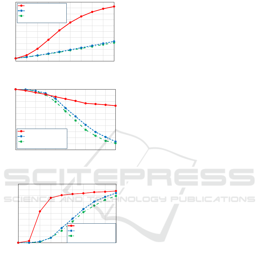
4.4 Results & Discussions

Figure 8 shows the results of all methods in each eva-

luation criterion.

As seen in the graphs, we can say that the com-

parative method outperforms the previous method in

the criterion of detected pedestrians though the im-

provement of the number of hit points is minor. From

this result, the use of orientation aware pedestrian li-

kelihood map proposed in this paper can slightly im-

prove the efﬁciency in the scan of pedestrians.

VISAPP 2019 - 14th International Conference on Computer Vision Theory and Applications

318

100

120

140

160

180

200

300 400 500 600 700 800 900 1,000 1,100 1,200

Number of hit points [point]

Number of laser irradiation [point]

Previous method

Comparative method

Proposed method

(Yamamoto et al., 2018)

(a) Hit points.

120

180

240

300

360

420

480

540

600

0 10 20 30 40 50 60 70 80 90 100

Number of detected pedestrians [person]

Threshold for pedestrian detection [point]

Previous method

Comparative method

Proposed method

(Yamamoto et al., 2018)

(b) Detected pedestrians.

Figure 8: Experimental results by two evaluation metrics.

120

180

240

300

360

420

480

540

600

300 400 500 600 700 800 900 1,000 1,100 1,200

Number of detected pedestrians [person]

Number of laser irradiation [point]

Previous method

Comparative method

Proposed method

(Yamamoto et al., 2018)

Figure 9: Transition of detected pedestrians using 40 points

as the threshold.

On the other hand, the proposed method outper-

forms both the comparative and the previous methods

in all evaluation criteria. Moreover, Figure 9 shows

the transition of detected pedestrians when the thres-

hold is set to 40 points. As seen in the graph, the

proposed method is able to obtain point-clouds from

pedestrians with less number of iteration than the ot-

her two methods.

Since the comparative and the previous methods

use average integration of the local likelihood map

by assuming that all measured points come from the

same object, the resultant pedestrian likelihood map

is blurred. On the other hand, the proposed method

controls the integration weight of the local likelihood

map according to the ratio of measured points coming

from the same object judged by depth-wise object se-

paration. Therefore, the proposed method could ge-

nerate the pedestrian likelihood map intensively fo-

cusing on pedestrian regions, and the performance of

the scan could be signiﬁcantly improved. From these

results, we conﬁrmed the effectiveness of the combi-

nation of orientation aware pedestrian likelihood map

and depth-wise object separation for improving the

efﬁciency of the scan.

Figure 11 shows the results of the proposed met-

hod and the previous method applied to the scene

shown in Fig. 10. From these results, we conﬁrmed

that the proposed method could efﬁciently control la-

ser directions focusing on a pedestrian, and could

achieve less laser irradiations than the previous met-

hod to dense obtain point-clouds from pedestrians.

5 CONCLUSIONS

In this paper, we proposed an efﬁcient pedestrian

scanning method based on the pedestrian likelihood

map constructed by integrating an orientation aware

local pedestrian likelihood map. Here, the local pede-

strian likelihood map is integrated according to the

weight related to the ratio of measured points that

comes from the same object. In the proposed met-

hod, pedestrian scanning is formulated as a problem

of stochastic sampling from the pedestrian likelihood

map, where pedestrians can be scanned progressively

by iterative scanning and map update.

To evaluate the performance of the proposed met-

hod, we conducted experiments by simulating the me-

chanism of an Active-scan LIDAR using the KITTI

dataset. As a result, the proposed method outperfor-

med comparative methods including the state-of-the-

art method.

Future work will include an improvement of the

local pedestrian likelihood map calculation, the deve-

lopment of a method to crop the pedestrians’ point-

clouds from point-clouds obtained by the proposed

method, and experiments with larger datasets.

ACKNOWLEDGEMENTS

Parts of this research were supported by MEXT,

Grant-in-Aid for Scientiﬁc Research.

Pedestrian Intensive Scanning for Active-scan LIDAR

319

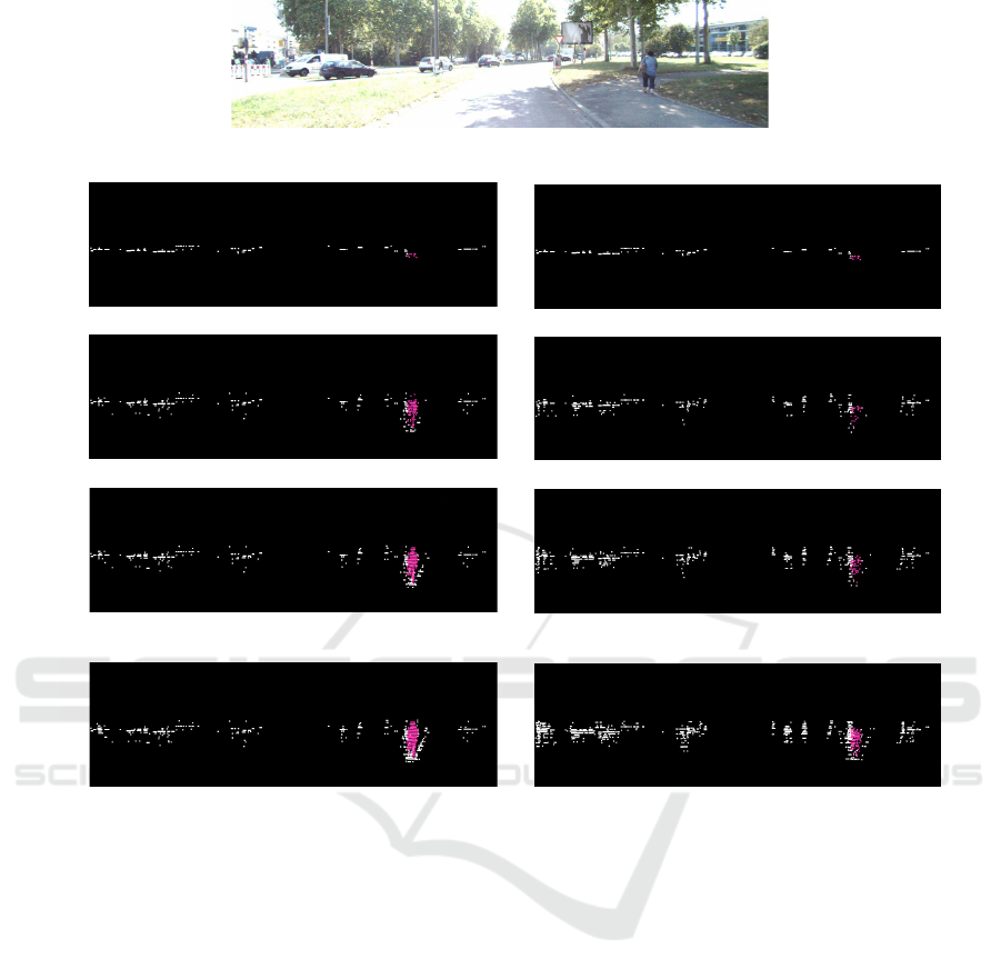
Figure 10: Sample scene in the KITTI dataset (Geiger et al., 2012).

⋯ ⋯ ⋯⋯

(a) Proposed method.

⋯ ⋯ ⋯⋯

(b) Previous method (Yamamoto et al., 2018).

Figure 11: Scanning results by the proposed method and the previous method (Yamamoto et al., 2018) applied to the scene in

Fig. 10. Pink dots represent pedestrians while white dots represent other objects. P

is a set of points obtained after the t-th

scan.

REFERENCES

Behley, J., Steinhage, V., and Cremers, A. (Nov. 2013).

Laser-based segment classiﬁcation using a mixture of

bag-of-words. In Proc. 2013 IEEE/RSJ Int. Conf. on

Intelligent Robots and Systems, pages 4195–4200.

Devroye, L. (1986). Non-uniform random variate genera-

tion. Springer.

Geiger, A., Lenz, P., and Urtasun, R. (June 2012). Are we

ready for autonoumous driving? The KITTI vision

benchmark suite. In Proc. 2012 IEEE Conf. on Com-

puter Vision and Pattern Recognition, pages 3354–

3361.

Kidono, K., Miyasaka, T., Watanabe, A., Naito, T., and

Miura, J. (June 2011). Pedestrian recognition using

high-deﬁnition LIDAR. In Proc. 2011 IEEE Intelli-

gent Vehicles Symposium, pages 405–410.

Maturana, D. and Scherer, S. (Sept. 2015). VoxNet: A 3D

convolutional neural network for real-time object re-

cognition. In Proc. 2015 IEEE/RSJ Int. Conf. on In-

telligent Robots and Systems, pages 922–928.

Tatebe, Y., Deguchi, D., Kawanishi, Y., Ide, I., Murase, H.,

and Sakai, U. (Jan. 2018). Pedestrian detection from

sparse point-cloud using 3DCNN. In Proc. 2018 Int.

Workshop on Advanced Image Technology, pages 1–4.

Wang, H., Wang, B., Liu, B., Meng, X., and Yang, G. (Feb.

2017). Pedestrian recognition and tracking using 3D

LIDAR for autonoumous vehicle. In J. of Robotics

and Autonoumous Systems, volume 88, pages 71–78.

Yamamoto, T., Shinmura, F., Deguchi, D., Kawanishi, Y.,

Ide, I., and Murase, H. (Jan. 2018). Efﬁcient pede-

strian scanning by active scan LIDAR. In Proc. 2018

Int. Workshop on Advanced Image Technology, pages

1–4.

Zhou, Y. and Oncel, T. (June 2018). VoxelNet: End-to-end

learning for point cloud based 3D object detection. In

Proc. 2018 IEEE Conf. on Computer Vision and Pat-

tern Recognition, pages 4490–4499.

VISAPP 2019 - 14th International Conference on Computer Vision Theory and Applications

320