Detection of Imaged Objects with Estimated Scales

Xuesong Li, Ngaiming Kwok, Jose E. Guivant, Karan Narula, Ruowei Li and Hongkun Wu

School of Mechanical and Manufacturing Engineering,

The University of New South Wales, NSW 2052, Australia

Keywords:

Computer Vision, Object Detection, Convolutional Neural Network.

Abstract:

Dealing with multiple sizes of the object in the image has always been a challenge in object detection. Pre-

deﬁned multi-size anchors are usually adopted to address this issue, but they can only accommodate a limited

number of object scales and aspect ratios. To cover a wider multi-size variation, we propose a detection

method that utilizes depth information to estimate the size of anchors. To be more speciﬁc, a general 3D

shape is selected, for each class of objects, that represents different sizes of 2D bounding boxes in the image

according to the corresponding object depths. Given these 2D bounding boxes, a neural network is used to

classify them into different categories and do the regression to obtain more accurate 2D bounding boxes. The

KITTI benchmark dataset is used to validate the proposed approach. Compared with the detection method

using pre-deﬁned anchors, the proposed method has achieved a signiﬁcant improvement in detection accuracy.

1 INTRODUCTION

Object detection is an important topic in computer vi-

sion community. Classical methods are usually de-

veloped based on handcrafted image features, such

as histograms of oriented gradient (HOG) (Dalal and

Triggs, 2005) and the deformable part model (DPM)

(Felzenszwalb et al., 2008). Recently, convolutional

neural network (CNN) has attracted much research at-

tention due to its astonishing performance for object

detection task(Ren et al., 2015; Liu et al., 2015; He

et al., 2017), whereby the image features are automa-

tically learned rather than handcrafted. These frame-

works (Ren et al., 2015; Liu et al., 2015; Redmon

et al., 2015) are widely used in image-based object

detection problems.

CNN-based object detection methods consist of

two main components: classiﬁcation and localization.

Classiﬁcation mainly relies on features of the target

object while localization regression depends on both

features and object sizes. CNN is able to ﬁnd scale-

invariant and object-speciﬁc features to identify the

objects; however, object sizes in the image are not

know a priori which makes detection tasks much more

difﬁcult than classiﬁcation tasks. In real-world appli-

cations, objects captured in an image usually have a

large scale variation such as shown in Fig.1; that ma-

kes object detection even more challenging. In order

to detect objects of different sizes, strategies including

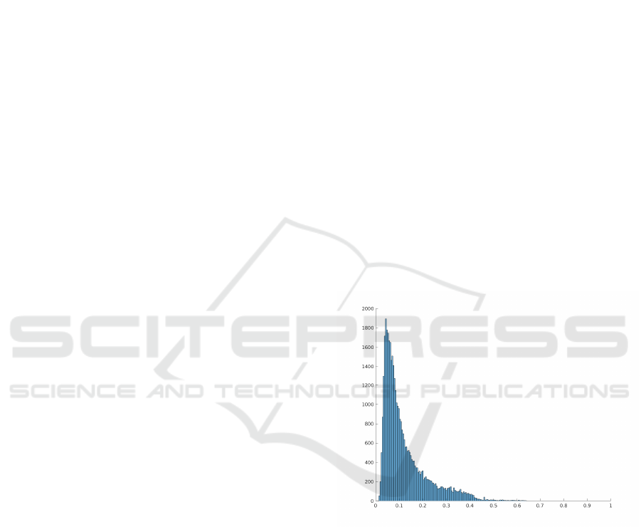
Object scale

Number of sample

Figure 1: Object scale histogram of KITTI, object scales

are depicted as the root square of object area divided by the

image size. The histogram bin size is 0.005.

image pyramid and multiple anchors were proposed.

Multi-size anchors are more commonly utilized to ﬁt

their corresponding objects, due to computation efﬁ-

ciency and cheap memory cost. For example, in the

Faster-RCNN (Ren et al., 2015), 9 discrete anchors

with 3 scales and 3 aspect ratios are adopted to handle

all object sizes. Then the most promising anchors are

the ones with similar sizes to the objects in the image,

and they are selected as inputs to the next stage clas-

siﬁer and regressor.

Those selected anchors are the discretized samples

from the continuous space of box scale and aspect ra-

Li, X., Kwok, N., Guivant, J., Narula, K., Li, R. and Wu, H.

Detection of Imaged Objects with Estimated Scales.

DOI: 10.5220/0007353600390047

In Proceedings of the 14th International Joint Conference on Computer Vision, Imaging and Computer Graphics Theory and Applications (VISIGRAPP 2019), pages 39-47

ISBN: 978-989-758-354-4

tio with a set of ﬁxed bins. Although using a larger

number of anchors can better represent the continu-

ous space, the corresponding increases in complexity

make regressors difﬁcult to learn scale-invariant fea-

tures and deep learning models expensive to train. On

the contrary, it is difﬁcult to ﬁnd a ﬁt for objects with

only a few anchors. Given size variations in the data-

set, the number of anchor scales and their aspect ratios

are important hyperparameters. The detection perfor-

mance is usually susceptible to improper settings of

these hyperparameters. In order to ﬁnd out how these

hyper-parameters affect ﬁnal performance and how to

select the optimal ones, we designed multiple control-

led experiments on KITTI benchmark dataset (Gei-

ger et al., 2012). We found that the set of designed

anchors for object detection should adequately cover

the continuous space of object scales and aspect ra-

tios, and simultaneously keeps a minimal number of

anchors. Subject to such a contradictory criterion, the

selection of the optimal hyperparameters is a challen-

ging task.

In order to satisfy both the requirements for desig-

ning anchors, we iteratively explore whether it is pos-

sible to estimate the continuous object scale that can

cover the whole scale space instead of pre-deﬁning

multiple discrete anchors with ﬁxed scales and as-

pect ratios. To acquire continuous scales, we utilize

the distance of the object with respect to the sen-

sor to estimate the coarse scale of the detected ob-

jects. A corresponding detection framework based

on CNN is also proposed to validate how estimated

scales can improve detection performance. To vali-

date our method, we conducted extensive evaluations

on the KITTI benchmark with a ﬁne-grained analy-

sis. Our proposed method can outperform state-of-

the-art with predeﬁned anchors while using the same

CNN backbone, especially on detecting difﬁcult ob-

jects. The proposed method can also be assembled

into multi-object detection algorithms with complex

detection frameworks (Ren et al., 2017) (Dai et al.,

2017). Our code is open-source and freely available

on github

There are three main works in our paper as follo-

wing.

• Designed controlled experiments to answer the

question of how the number of predeﬁned anchors

affects the detection performance.

• Proposed a detection method based on estimated

size of objects.

• Conducted massive experiments on the KITTI

benchmark to validate our method.

Main open-source code can be found: https://github.

com/Benzlxs/Object detection estimated sclales

The rest of the paper is organized as follows.

Section 2 is an introduction to the related work, follo-

wed by Section 3 which illustrates how multiple an-

chors affect detection accuracy. Our proposed de-

tection method is presented in Section 4. Experi-

ments of the proposed method are given in Section 5.

Section 6 concludes our main work and summarizes

the contributions of this paper.

2 RELATED WORK

2.1 Mutli-size Detectors

Scale-space theory (Lindeberg, 1990) is a vital and

fundamental theory in signal processing, and signiﬁ-

cant research has been devoted to this ﬁeld. Multi-

size detectors (Ren et al., 2015) are usually utilized

to address multi-scale of objects. Multi-size detec-

tors take one-size input and apply multi-size detec-

tors to detect their corresponding objects (Ren et al.,

2015; Lin et al., 2016; He et al., 2016). The Faster-

RCNN (Ren et al., 2015) implements detection on the

ﬁnal feature map using 9 different anchors with 3 dif-

ferent sizes and 3 different aspect ratios. Each an-

chor can represent one size detector that ﬁnds objects

with similar sizes. However, the ﬁnal feature map

is usually at a low resolution with high-level seman-

tic information, which makes small objects detection

very challenging. To improve small objects detection,

the feature pyramid network is proposed to propagate

high-level semantic information in deeper layers back

to shallower layers with high-resolution maps; Small

objects are mainly detected from fused shallower fea-

ture maps (Lin et al., 2016). The recurrent rolling net-

work extends feature pyramid network by using a re-

current neural network to fuse feature maps from dif-

ferent layers and integrate context information (Ren

et al., 2017). However, even pyramid feature maps

may not be useful for detecting small-size object since

high-level information does not contain the semantic

feature on small objects. Therefore, to increase the ﬁ-

nal feature map resolution, by upsampling the image,

has become the most common practical technique to

detect small objects instead of building an image py-

ramid (He et al., 2016).

Some methods are proposed to change the size

of the receptive ﬁeld to accommodate multi-scale ob-

jects, which includes the dilated and deformable con-

volutional network (Dai et al., 2017; Yu and Kol-

tun, 2015). Transformation parameters are learned

by a network, similar to STN (Spatial Transformer

Networks) (Jaderberg et al., 2015), by building the

STN to perform an afﬁne transformation on input fe-

VISAPP 2019 - 14th International Conference on Computer Vision Theory and Applications

atures for the classiﬁcation task. These methods re-

quire the CNN backbone in the detection model to le-

arn scale-invariant features and utilize one detection

head to do classiﬁcation and regression on all scale

objects together. Contrary to this, two sub-networks

are used to predict multi-scale objects independently

(Li et al., 2015), and every sub-network handles ob-

ject within its scale range. Such kind of indepen-

dent prediction is made at layers of different resolu-

tions. MSC-CNN (Cai et al., 2016) claims that re-

ceptive ﬁled of CNN should be consistent with the

size of objects, and design algorithms to detect dif-

ferent scale objects on feature maps of multiple re-

solutions. Every resolution represents one receptive

ﬁeld size on which objects within certain scale ranges

are found. Deep learning models can manage to learn

scale-invariant representations when the scales varia-

tion is not large but still suffers from extremely small

and large scale variations of objects. On the other

hand, scale-speciﬁc methods with an image pyramid

can handle all scales well. To combine the advantages

of scale-variant and scale-invariant methods, coarse

image pyramids are built (Singh and Davis, 2017; Hu

and Ramanan, 2016) from 3 levels as input. Every

level in the pyramid corresponds to one detection mo-

del which is just required to deal with a ﬁxed range of

scales instead of all object scales in the training data-

set. Such methods usually achieve the state-of-the-art

performance where each object detector focuses only

on objects within certain scale ranges.

All multi-scale detection methods mentioned in

this section rely on manually predeﬁning anchors.

Every anchor is designed to cover one size of target

objects and its region in the image will be pooled into

a ﬁxed shape as scale-invariant feature representati-

ons, so hyperparameters of these anchors are vital for

detection performance. Instead of heavily relying on

tuning the hyperparameters of anchors, we proposed a

detection method in this work that uses estimated an-

chors to conver all continuous scales and aspect ratios

of detected objects.

2.2 Depth based Detection Methods

Depth information is already available in many ap-

plications. To take advantage of the depth data for

object detection, common methods compress 3D in-

formation into 2D information on which the CNN is

applied directly. 3D point cloud is encoded into a

cylindrical-like image where every valid element car-

ries 2-channel data so that the 2D image can inherit

all the information from the 3D point cloud (Li et al.,

2016). The 2D CNN is then used to process such kind

of 2D image to detect the object. However, such kind

of data representation fails to achieve decent detection

performance. To improve accuracy further, The work

in (Chen et al., 2016) convert 3D point cloud into

birdview representation which includes many height

maps, a density map, and an intensity map; based on

this representations, the CNN is then applied to pro-

pose 3D object candidates. These methods actually

regard point clouds as one extra image channel and

are similar with ideas used to deal with RGBD data

(Gupta et al., 2014). In this work, we employ raw

depth data to estimate coarse scale in an efﬁcient and

simple manner instead of encoding depth information

into some feature maps. Estimated scales can remove

the need for manually predeﬁning anchors and are

able to cover all possible continuous scales.

3 MULTIPLE ANCHORS

Predeﬁned multi-scale anchors are crucial to the per-

formance of the detection method. This section des-

cribes how these anchors affect detection results and

how to select optimal predeﬁned anchors.

3.1 Scales and Aspect Ratios

Predeﬁned anchors are a set of boxes with different si-

zes



) : 1 6 i 6 N



in which w

and h

are width

and height of the box respectively, and N is the num-

ber of predeﬁned anchors. The size of an anchor is

deﬁned by its scale and aspect ratio that denote the an-

chor area and the ratio between box height and width.

At each sliding-window location (x

), N proposal

boxes



) : 1 6 i 6 N,1 6 j 6 W × H



where W and H are the size of feature map will be

predicted by the network. Therefore, H ×W × N pro-

posals will be generated by the region proposal net-

work. Each anchor size, (w

), can be calculated

according to equation. 1 and 2.

(1)

= S

(2)

Scales



: 1 6 k 6 K



are another set of pre-

deﬁned parameters. Every S

represents one scale of

the anchor and can be calculated as the root square of

the anchor region in the image coordinate.



: 1 6

j 6 J



is the set of aspect ratios, and J is the number

of predeﬁned aspect ratio for every scale. As shown

in Equ. 1 and 2, every scale will be expanded to J

anchors, which have the same area of different ratios

between height and width, in order to handle various

poses of the same object in the image. The number

Detection of Imaged Objects with Estimated Scales

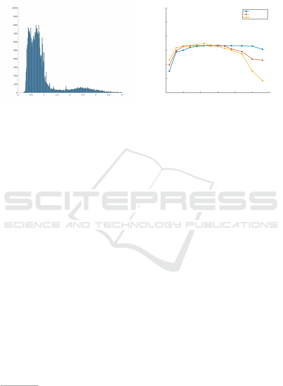
Aspectio ratio(H/W)

Number of samples

Figure 2: Object aspect ratio histogram of KITTI dataset.

Aspect ratios are calculated by dividing H by W of the box

size. Histogram bin size is 0.001.

of anchors N is K × J, and H ×W × K × J proposal

boxes will be generated.

3.2 Anchor Selection

Variables S

and R

are very important user-deﬁned

hyperparameters. To understand how these hyper-

parameters affect the ﬁnal detection performance,

we conduct controlled experiments on KITTI dataset

(Geiger et al., 2012). The object scale and aspect ratio

histograms can be found in Fig. 1 and 2. The domain

of scale and aspect ratio variation are [0.0, 0.64] and

[0.25,10.56] respectively. In our experiments, we uni-

formly sample different scales in [0.02,0.54] instead

of the full range, because the 99.5% of the objects in

the training data reside in this range and the full range

with extremely large and small scale will bring very

heavy experimental workload. Similarly, the chosen

sampling range of aspect ratios is between [0.25,4.0],

in which 99.5% of all the objects can be covered. The

Faster-RCNN (Ren et al., 2015) with VGG16 net-

work backbone (Simonyan and Zisserman, 2014) is

employed in our experiments

. Results are plotted in

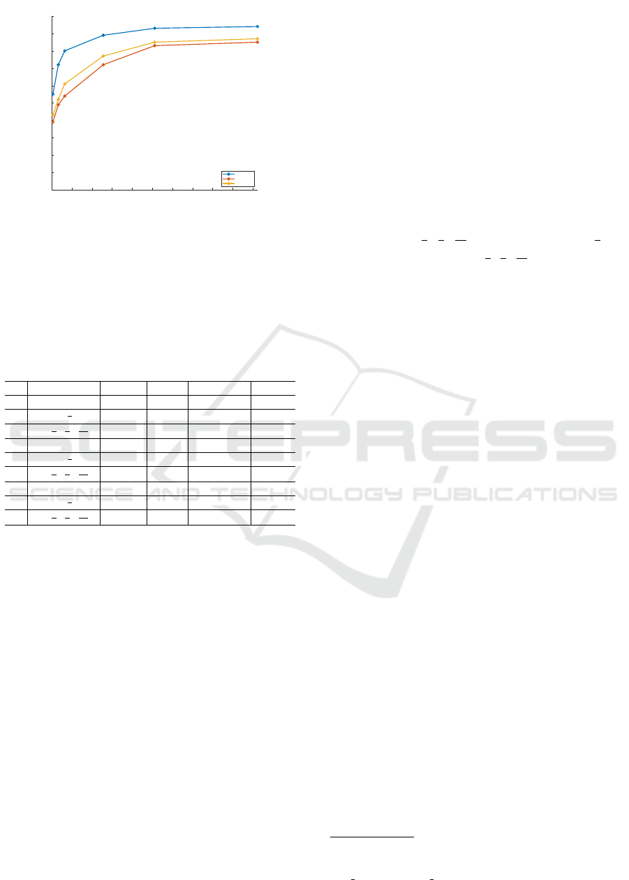
Fig. 3.

From the Fig. 3, we ﬁnd that three anchors set-

tings, (K = 3,R = 25), (K = 5,R = 15) and (K =

7,R = 11), can respectively achieve the best perfor-

mance among their anchor sets with the same aspect

ratios (K) but different scales (R). The interesting

phenomenon is that the total number of anchors in

these three sets is very similar and close to 75. When

the anchor number is small, less than 75, the detection

accuracy is proportional to the anchor number. It is

because more anchors can help to better cover the

Experimental code and results can be found https://

github.com/Benzlxs/TFFRCNN

0 5 10 15 20 25 30

Number of scale

100

Detection mAP

3-aspect-ratio

5-aspect-ratio

7-aspect-ratio

Figure 3: Comparison of detection mAP against different

combinations of scales and aspect ratios. The Detection

mAP is the mean average detection precision of car, cyclist

and pedestrian of all degree of difﬁculties.

continuous domain of all object sizes, and every an-

chor just needs to handle a small range of size varia-

tion which reduces learning difﬁculties of the region

proposal network. If the number of anchors is too

large, the detection accuracy will be inversely propor-

tional to the anchor number. The reason is that a lar-

ger number of possible predeﬁned boxes will lead to a

signiﬁcant imbalance between the positive and nega-

tive examples, and easy negative examples can over-

whelm the training of region proposal network which

may in turn lead to degenerate models. Another rea-

son is that the number of convolution prediction ﬁlters

increases linearly with the number of anchors; toget-

her with the ﬁxed number of training labels, a large

proportion of the prediction ﬁlters are unable to get

enough training. Besides, as the number of prede-

ﬁned anchors increases, the computational and me-

mory cost will also increase and more training time

will be required. It is concluded that predeﬁned an-

chors should be able to cover all possible scales of

objects, but their numbers should be as small as pos-

sible.

It is difﬁcult to predeﬁne anchors that satisfy both

the requirements mentioned above. The common way

is to conduct trial-and-error experiments to ﬁnd the

optimal number for one dataset, which can be com-

putationally demanding and time-consuming. There-

fore, we introduce the depth information into the net-

work in order to reduce the required number of an-

chors. The depth information is utilized to estimate

the coarse size of the objects that ca cover the conti-

nuous scale and aspect ratio ranges at the same time.

For every location, only a few anchor boxes are gene-

rated according to the number of target object types

and real size variations.

VISAPP 2019 - 14th International Conference on Computer Vision Theory and Applications

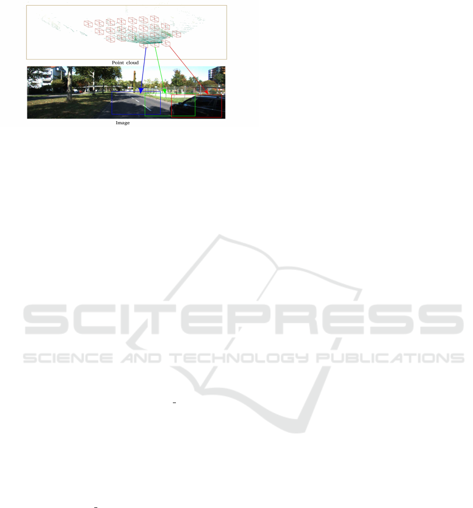
Figure 4: Examples of projection from P

to P

. The top

image is 3D bounding boxes of P

in point cloud coor-

dinate, and the bottom one is 2D bounding boxes of their

corresponding P

4 DETECTION WITH

ESTIMATED ANCHOR

In many real-world applications, like the driverless

car and indoor service robot, depth information is

there for other purposes and can be obtained easily

by depth sensors such as stereo camera or Lidar. The

depth information can decide the object location in

3D space, and coarse 3D size of detected objects can

be predeﬁned, for example, 4.2 × 1.8 × 1.6 m

can

coarsely represent the 3D bounding box of a sedan.

Given calibration parameters between the depth sen-

sor and camera, the 3D bounding box can be projected

into a 2D region in image coordinate, and the 2D re-

gion can be used to represent a coarse scale of the de-

tected object. Thousands of projected regions will be

generated and used to crop object features from light

feature map compressed from conv5 3 of VGG16.

RoI (Region of Interest) pooling is implemented to

convert every region feature into ﬁxed shape as scale-

invariant feature representations. The scale-invariant

network consisting of two fully connected layers is

used to do coarse classiﬁcation and regression to ﬁnd

valuable proposals. It has the similar function with

the region proposal network. Selected regions are

then used to do cropping and RoI pooling on the thick

feature map conv5 3 for the second-stage classiﬁca-

tion and regression which includes three-layers of the

fully connected network.

Based on the observation of the process described

in the previous section, the proposed detection met-

hod will estimate a coarse region size of the object,

), and applies it to enhance the performance of

object detection. In this section, inference about ob-

ject size and how to integrate scale into the CNN fra-

mework for object detection will be presented.

4.1 Anchor Estimation

The distance between the observer and objects can al-

most tell their scales in the image, so scale for dif-

ferent objects can be coarsely estimated from their

depth map. Without predeﬁning a set of possible an-

chors, we utilize depth to estimate the coarse size of

target objects. Given image coordinates and depth

data, 3D point cloud can be generated using simple

afﬁne transformation. Some noisy points represen-

ting the sky region will be removed. Thousands of

3D bounding boxes that can represent the coarse 3D

size of detected objects are employed to wrap all se-

lected points. These 3D bounding boxes are projected

back into image coordinate to ﬁnd the coarse sizes of

the anchors.

We validate our method using KITTI dataset

where point cloud data is available. The 3D space

range for sampling 3D bounding boxes are [0,70] m

along x axis and [−40,40] m along y axis under Lidar

coordinate convention. We slide these 3D bounding

boxes along x and y axes with 0.4 m intervals on the

road plane which can easily be estimated by random

sample consensus. 3D boxes are ﬁltered out by remo-

ving those in which the number of points is less than

4. Then, 8 corner points P

of remaining boxes will

be projected back to points P

in image coordina-

tes according to Equ.3, where R is the rotation matrix

and T is the transformation matrix. Calibration para-

meters are provided in the KITTI dataset.

= R × P

+ T (3)

Projected boxes in the image coordinate can be

employed as the coarse size of the anchor, such as in

Fig. 4. Instead of sliding a ﬁxed set of anchors over

every point in the feature map as in Faster-RCNN, we

just generate a smaller number of region boxes on in-

teresting points, about 40,000 of them, while Faster-

RCNN with 15 anchors will generate about 200, 000

region boxes.

4.2 Detection Network

CNN has been widely and successfully used to ex-

tract features from an image for object detection and

classiﬁcation, and it is adopted to generate feature

maps in our detection method. Based on feature maps,

fully connected layers are employed to do classiﬁca-

tion and regression. The method pipeline is depicted

in Fig. 5.

The VGG16 (Simonyan and Zisserman, 2014) are

used to generate feature maps from the input image.

Numerous 2D boxes N

roi

will be estimated from depth

information according to the method described in the

Detection of Imaged Objects with Estimated Scales

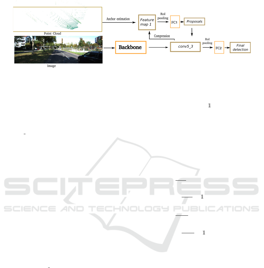
Figure 5: The proposed detection framework. Backbone is pretrained VGG16.

previous section. Usually, the last layer of feature

maps has a large number of channels (512 in VGG16).

If we crop features from the estimated boxes directly

on a wide feature map, the large number of scale

boxes will be memory-intensive and computationally

expensive. Therefore, by using 1 × 1 convolutional

layers, we compress the last layer of feature maps,

the conv5 3 of VGG16, into a thin feature map, Fe-

ature map 1 in the Fig.5, with 32 channels of the

same width and height. Compressed feature maps

are designed to select primary features for region pro-

posal network. Every estimated region box will be

used to crop its corresponding feature on Feature map

1 into 5 × 5 × 32 scale-invariant features, also cal-

led ROI pooling operation. Then, features are con-

nected with light-weight FC1 which consists of two

fully connected layers with 512 neurons per layer.

The FC1 plays the same role as the region proposal

network in the Faster-RCNN (Ren et al., 2015); it

will perform coarse classiﬁcation with output N

roi

2( f oreground/background) and regression of boxes

with output N

roi

×4. N

rpn

will be selected from N

roi

a mini-batch to train the FC1 network. All predicted

boxes are post-processed by non-maximum suppres-

sion (NMS) to select the top N

prop

proposals. Since

the number of proposals is small, selected proposals

are used to do RoI pooling directly on the last layer of

the backbone conv5 3. Then, 7 × 7 × N

prop

features

are produced and connected to FC2 which contains

three layers of the fully connected layers with 2048

neurons each. The FC2 will generate ﬁnal detection

results, N

prop

×C (the number of category) for classi-

ﬁcation and N

prop

× 4 for bounding box regression.

The loss function is deﬁned in Equ. 4, 5 and 6,

which consists of two terms, L

rpn

and L

. L

rpn

used to train the region proposal network, FC1, while

is for the second-stage reﬁneing network, FC2.

Loss of the whole detection network is the sum of

these two term with weighting parameter α. L

cls

the cross entropy between predicted categories and

corresponding labels, and L

reg

is the smooth

loss

function (Ren et al., 2015). p

and t

are the outputs

of classiﬁcation and regression network; p

i∗

and t

i∗

are their corresponding ground truths. A set of pro-

posals N

rpn

, 512 in our conﬁguration, is selected from

roi

. When calculating the regression loss, only po-

sitive labels will be counted ( indicates that there is

a positive label). N

pos

rpn

represents the number of po-

sitive labels, and N

prop

, 1024 in our conﬁguration, is

the number of samples we selected for the second-

stage network FC2. These hyperparameters are se-

lected according to numerous experiments in the next

section. The AdamOptimizer (Kingma and Ba, 2014)

is employed to train our network end-to-end.

all

= L

rpn

+ αL

(4)

rpn

∑

cls

rpn

, p

i∗

rpn

)

pos

rpn

∑

ob j

reg

rpn

i∗

rpn

)

(5)

prop

∑

cls

, p

j∗

)

pos

prop

∑

ob j

reg

j∗

)

(6)

5 EXPERIMENTS

The proposed method is evaluated on the KITTI ben-

chmark, which includes 7481 training and 7518 tes-

ting sets of high-resolution images. LIDAR laser data

is also available. Since the ground truth of the tes-

ting dataset is not publicly available, we split the trai-

ning dataset in the 3:1 ratio for training and valida-

tion respectively. These are then used to conduct

comparative experiments for the purpose of deducing

how the hyperparameters affect the detection perfor-

mance. The 0.7 IoU threshold for the car and 0.5 IoU

threshold both for pedestrian and cyclist are used to

calculate mean Average Precision (mAP). Lastly, the

adequately-trained network model with optimal hy-

perparameters is deployed to process the testing data-

set and the detection result is submitted to the bench-

VISAPP 2019 - 14th International Conference on Computer Vision Theory and Applications

0 200 400 600 800 1000 1200 1400 1600 1800 2000

Number of proposals

0.1

0.2

0.3

0.4

0.5

0.6

0.7

0.8

0.9

Recall

car

pdestrain

cyclist

Figure 6: Proposal recall on the KITTI validation set for

three classes.

mark site to compare against the Faster-RCNN met-

hod.

Table 1: Experiments on how to select predeﬁned 3D boun-

ding boxes, the detection performance is mAP(%) of easy,

moderate and hard categories. The deﬁnition of easy, mode-

rate and hard objects can be found in the benchmark (Geiger

et al., 2012).

K orientation ∼ N

roi

car pedestrian cyclist

1 [0] 5,000 76.48 68.12 60.78

1 [0,

] 10,000 85.64 71.29 70.36

1 [0,

3π

] 20,000 89.12 72.01 74.51

2 [0] 10,000 80.65 71.85 63.62

2 [0,

] 20,000 88.23 73.96 74.82

2 [0,

3π

] 40,000 91.68 74.00 76.45

3 [0] 15,000 81.87 72.93 63.80

3 [0,

] 30,000 90.03 74.03 74.64

3 [0,

3π

] 60,000 91.51 74.09 76.51

For data augmentation, horizontally ﬂipping and

color jittering are used to increase the number of trai-

ning dataset. The data is augmented by a factor of

three such that its size is three times as big as the size

of the original dataset. The whole detection network

is trained in an end-to-end manner. The AdamOpti-

mizer(Kingma and Ba, 2014) is conﬁgured with an

initial learning rate of 0.0005 and exponential decay

factor of 0.6 for every 40,000 iterations.

5.1 Hyperparamters Selection on the

Validation Set

The number of estimated anchors N

roi

and the number

of proposals N

prop

, are important hyperparameters for

our detection framework. For the number of estima-

ted anchors N

roi

, it consists of valid non-road point

cloud and predeﬁned 3D template bounding boxes of

different sizes and orientations. As for box sizes, we

use the k-means clustering method to do clustering

on 3D bounding box size of all training labels and

calculate average box size of every cluster. For ex-

ample, if we just use one size of the 3D bounding

box for the car and setting k=1, the clustered size

result is [3.884(length), 1.629(width),1.526(height)]

m. While if we use two sizes of 3D bounding

box for car and setting k=2, the clustered sizes are

[3.539,1.599,1.506] m and [4.229,1.658,1.546] m.

Experimental results are shown in Table 1, from

which we can ﬁnd that increasing the orientation and

size (k) number will improve detection performance

until N

roi

is large, like over ∼ 30,000, while large N

roi

will make training much slower and consume more

memory. Considering the tradeoff between efﬁciency

and accuracy, we ﬁnally select size clusters k=2 and

orientations [0,

3π

] for car; k=1 and [0,

] for

pedestrian; and k=2 and [0,

3π

] for cyclist in our

framework.

For the number of proposals N

prop

, we output all

the proposals from region proposal network and do

NMS with the IoU threshold of 0.8. The top N

prop

proposals are saved to calculate the recall. The expe-

rimental results are shown in Fig 6, from which we

can ﬁnd that when N

prop

the is over 1024, the recall

barely increases. Since smaller N

prop

consumes less

memory and speeds up the training procedure, N

prop

of 1024 is chosen for the experiments.

5.2 Evaluation on the Test Set

Results

are shown in Table 2, Fig 7 and 8. We

conduct comparisons with the Faster-RCNN, for both

of our method and Faster-RCNN employ the same

VGG16 backbone (Simonyan and Zisserman, 2014),

but different methods to determine the object scale

and aspect ratio. On the KITTI benchmark, results

of Faster-RCNN with 70 anchors are available for all

objects, while Faster-RCNN with 9 anchors is only

evaluated on car detection. For car detection, results

of Faster-RCNN with 70 and 9 anchors are compa-

red with our method. We can ﬁnd that increasing the

number of anchors can signiﬁcantly enhance the de-

tection accuracy. The detection performance of the

Faster-RCNN in detecting the car objects peaks when

the anchor number reaches 70. Our proposed met-

hod with the estimated scales, on the other hand, can

gain similar detection accuracy on the easy category.

However, on moderate and difﬁcult categories, esti-

mated scales can help to ﬁnd the anchor size clo-

sest to the detected object, which reduces the difﬁ-

culties of regressing locations of moderate and difﬁ-

cult objects. For pedestrian and cyclist detection, only

Testing results can be found in the KITTI object

detection leaderboard http://www.cvlibs.net/datasets/kitti/

eval object.php?obj benchmark=2d

Detection of Imaged Objects with Estimated Scales

0.2

0.4

0.6

0.8

0 0.2 0.4 0.6 0.8 1

Precision

Recall

Car

Easy

Moderate

Hard

0.2

0.4

0.6

0.8

0 0.2 0.4 0.6 0.8 1

Precision

Recall

Cyclist

Easy

Moderate

Hard

0.2

0.4

0.6

0.8

0 0.2 0.4 0.6 0.8 1

Precision

Recall

Pedestrian

Easy

Moderate

Hard

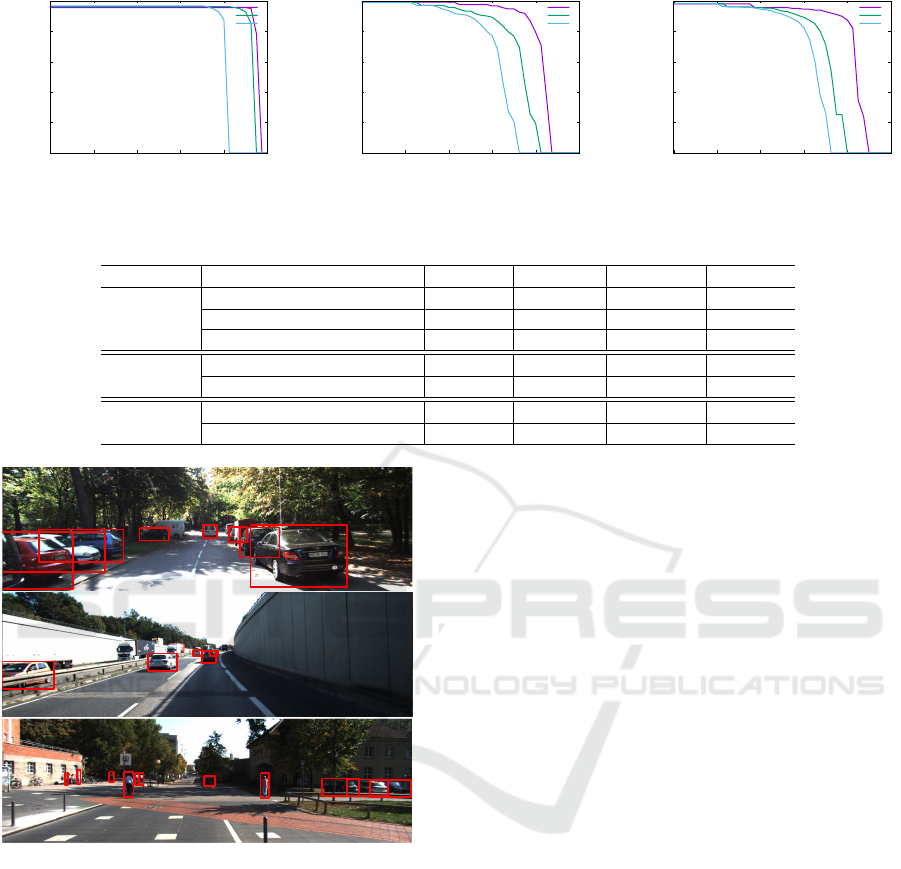
Figure 7: Precision recall curves for object detection on KITTI test set.

Table 2: Detailed result for object detection on KITTI test set, given in terms of average precision (AP).

Object Method mAP Easy Moderate Hard

Car

Proposed method 84.08 % 86.82% 87.10% 78.32%

Faster-RCNN (70 anchors) 79.01 % 87.9 % 79.11 % 70.19%

Faster-RCNN (9 anchors) 54.72% 62.31% 56.58 % 45.27 %

Cyclist

Proposed method 69.88 % 78.51 % 69.80 % 61.32 %

Faster-RCNN (70 anchors) 63.22 % 71.41 % 62.81 % 55.44 %

Pedestrian

Proposed method 69.16 % 77.95 % 67.25 % 62.28%

Faster-RCNN (70 anchors) 68.48 % 78.35 % 65.91 % 61.19 %

0.99

0.66

0.68

0.33

0.59

0.91

0.67

0.92

0.56

0.91

0.67

0.92

0.56

Figure 8: Some samples of detection results on KITTI test

set.

Faster-RCNN with 70 anchors is evaluated on the tes-

ting dataset and compared with our method. There

are 6.66 % and 0.68 % accuracy gains in the mAP are

achieved for the cyclist and the pedestrian category re-

spectively. One explanation is that cyclists have much

larger variation in scale and aspect ratio than the pede-

strians, therefore, estimated anchors brings more ad-

vantages than predeﬁned anchors for the cyclists.

6 CONCLUSION

Inexact multiple scales and aspect ratios are obstacles

in the detection of all objects in the image. Classi-

cal methods use predeﬁned anchors to solve this pro-

blem, but the discrete and sparse anchor samples are

not able to cover all scales and aspect ratios.The sim-

ple solution of increasing the number of anchors is

infeasible since a large number of anchors hinders the

training of CNN. To ﬁnd the optimal size of anchors,

we proposed to use depth information to estimate a

coarse scale of objects and designed the correspon-

ding detection framework. The proposed method can

achieve a signiﬁcant improvement compared with the

method using a similar backbone and predeﬁned an-

chors. However, using the depth information to esti-

mate coarse anchor sizes makes it unfeasible for many

applications where the depth information is not avai-

lable. Currently, there are researches indicating the

neural network has been successfully used to predict

object depths from a single image. Our future rese-

arch will endeavor to estimate estimate coarse and

continuous anchor sizes from a single image.

REFERENCES

Cai, Z., Fan, Q., Feris, R. S., and Vasconcelos, N. (2016). A

uniﬁed multi-scale deep convolutional neural network

for fast object detection. CoRR, abs/1607.07155.

Chen, X., Ma, H., Wan, J., Li, B., and Xia, T. (2016). Multi-

view 3d object detection network for autonomous dri-

ving. arXiv preprint arXiv:1611.07759.

Dai, J., Qi, H., Xiong, Y., Li, Y., Zhang, G., Hu, H., and

Wei, Y. (2017). Deformable convolutional networks.

CoRR, abs/1703.06211.

Dalal, N. and Triggs, B. (2005). Histograms of oriented gra-

dients for human detection. In Computer Vision and

VISAPP 2019 - 14th International Conference on Computer Vision Theory and Applications

Pattern Recognition, 2005. CVPR 2005. IEEE Com-

puter Society Conference on, volume 1, pages 886–

893. IEEE.

Felzenszwalb, P., McAllester, D., and Ramanan, D. (2008).

A discriminatively trained, multiscale, deformable

part model. In Computer Vision and Pattern Recog-

nition, 2008. CVPR 2008. IEEE Conference on, pages

1–8. IEEE.

Geiger, A., Lenz, P., and Urtasun, R. (2012). Are we re-

ady for autonomous driving? the kitti vision bench-

mark suite. In Computer Vision and Pattern Recogni-

tion (CVPR), 2012 IEEE Conference on, pages 3354–

3361. IEEE.

Gupta, S., Girshick, R. B., Arbelaez, P., and Malik, J.

(2014). Learning rich features from RGB-D ima-

ges for object detection and segmentation. CoRR,

abs/1407.5736.

He, K., Gkioxari, G., Doll

ar, P., and Girshick, R. B. (2017).

Mask R-CNN. CoRR, abs/1703.06870.

He, K., Zhang, X., Ren, S., and Sun, J. (2016). Deep resi-

dual learning for image recognition. In Proceedings of

the IEEE conference on computer vision and pattern

recognition, pages 770–778.

Hu, P. and Ramanan, D. (2016). Finding tiny faces. CoRR,

abs/1612.04402.

Jaderberg, M., Simonyan, K., Zisserman, A., and Kavukcu-

oglu, K. (2015). Spatial transformer networks. CoRR,

abs/1506.02025.

Kingma, D. P. and Ba, J. (2014). Adam: A method for

stochastic optimization. CoRR, abs/1412.6980.

Li, B., Zhang, T., and Xia, T. (2016). Vehicle detection

from 3d lidar using fully convolutional network. arXiv

preprint arXiv:1608.07916.

Li, J., Liang, X., Shen, S., Xu, T., and Yan, S. (2015). Scale-

aware fast R-CNN for pedestrian detection. CVRR,

abs/1510.08160.

Lin, T., Doll

ar, P., Girshick, R. B., He, K., Hariharan, B.,

and Belongie, S. J. (2016). Feature pyramid networks

for object detection. CoRR, abs/1612.03144.

Lindeberg, T. (1990). Scale-space for discrete signals. IEEE

Transactions on Pattern Analysis and Machine Intel-

ligence, 12(3):234–254.

Liu, W., Anguelov, D., Erhan, D., Szegedy, C., Reed, S. E.,

Fu, C., and Berg, A. C. (2015). SSD: single shot mul-

tibox detector. CoRR, abs/1512.02325.

Redmon, J., Divvala, S. K., Girshick, R. B., and Farhadi, A.

(2015). You only look once: Uniﬁed, real-time object

detection. CoRR, abs/1506.02640.

Ren, J., Chen, X., Liu, J., Sun, W., Pang, J., Yan, Q., Tai,

Y.-W., and Xu, L. (2017). Accurate single stage detec-

tor using recurrent rolling convolution. arXiv preprint

arXiv:1704.05776.

Ren, S., He, K., Girshick, R., and Sun, J. (2015). Faster

r-cnn: Towards real-time object detection with region

proposal networks. In Advances in neural information

processing systems, pages 91–99.

Simonyan, K. and Zisserman, A. (2014). Very deep con-

volutional networks for large-scale image recognition.

CoRR, abs/1409.1556.

Singh, B. and Davis, L. S. (2017). An analysis of

scale invariance in object detection - SNIP. CoRR,

abs/1711.08189.

Yu, F. and Koltun, V. (2015). Multi-scale context aggrega-

tion by dilated convolutions. CoRR, abs/1511.07122.

Detection of Imaged Objects with Estimated Scales