Equivalence of Turn-Regularity and Complete Extensions
Alexander M. Esser
Fraunhofer Institute for Intelligent Analysis and Information Systems IAIS, Sankt Augustin, Germany
Keywords:
Graph Drawing, Orthogonal Drawing, Compaction, Turn-Regularity, Complete Extension.
Abstract:
The aim of the two-dimensional compaction problem is to minimize the total edge length or the area of an
orthogonal grid drawing. The coordinates of the vertices and the length of the edges can be altered while all
angles and the shape of the drawing have to be preserved. The problem has been shown to be NP-hard.
Two commonly used compaction methods are the turn-regularity approach by (Bridgeman et al., 2000) and
the approach by (Klau and Mutzel, 1999) considering complete extensions. We formally prove that these
approaches are equivalent, i. e. a face of an orthogonal representation is turn-regular if and only if there exists
a unique complete extension for the segments bounding this face.
1 INTRODUCTION
The compaction problem has been one of the chal-
lenging tasks in graph drawing for many years, as
orthogonal drawings suffered from insufficient com-
paction algorithms, and as compaction plays an im-
portant role for various applications.
To give a practical example: In VLSI design the
vertices of a graph represent electrical components,
such as transistors, contacts, or logic gates, while the
edges represent wires connecting these components
(Lengauer, 1990). Minimizing the area, width, height
or total edge length of such an orthogonal drawing
representing a chip layout, with a certain distance be-
tween all the electrical components though, is essen-
tial for this use case.
Schematic drawings are almost always subject to
size limitations. Thus, apart from VLSI design, com-
paction is important in many other contexts in infor-
mation visualization. The types of drawings and do-
mains range from UML diagrams in the area of soft-
ware engineering, via entity-relationship diagrams for
database management, through to subway maps (Ba-
tini et al., 1984), (Batini et al., 1986), (Tamassia,
1987), (Tamassia et al., 1988), (Di Battista et al.,
1995), (Eiglsperger, 2003), (Eiglsperger et al., 2003).
1.1 Topology-Shape-Metrics Scheme
Orthogonal grid drawings are usually generated in
three phases, according to the topology-shape-metrics
scheme (Batini et al., 1986):
In the first phase, the graph is planarized, i. e. a
plane embedding is computed while the number of
crossings is minimized. For non-planar graphs, edge
crossings are replaced by artificial vertices.
In the second phase, the orthogonal shape of the
drawing is determined. This means that bends along
the edges and the angles between the edges around
each vertex are determined while the number of bends
is minimized.
In the third phase, the drawing is compacted.
Here, the coordinates of the vertices are mapped to a
grid and the length of each edge is determined while
the shape of the drawing is preserved. The goal of
the compaction phase is to minimize the total edge
length of the drawing. Patrignani (2001) has proven
this problem to be NP-hard; Bannister and Eppstein
(2012) have given inapproximability results for non-
planar drawings.
1.2 State-of-the-Art
Since the orthogonal compaction problem is NP-hard,
for a long time one-dimensional compaction heuris-
tics were applied. These one-dimensional heuristics
transform the two-dimensional compaction problem
into two one-dimensional problems, and solve them
by applying minimum-cost flow techniques (Tamas-
sia, 1987), (Eiglsperger et al., 2001). In one dimen-
sion – either the x- or y-dimension – the orthogonal
drawing is considered to be fixed, while in the other
dimension the coordinates of the vertices can be alte-
red. This, in general, does not lead to optimal results.
Esser, A.
Equivalence of Turn-Regularity and Complete Extensions.
DOI: 10.5220/0007353500390047
In Proceedings of the 14th International Joint Conference on Computer Vision, Imaging and Computer Graphics Theory and Applications (VISIGRAPP 2019), pages 39-47
ISBN: 978-989-758-354-4
Copyright
c
 2019 by SCITEPRESS – Science and Technology Publications, Lda. All rights reserved
39

(a) (b)
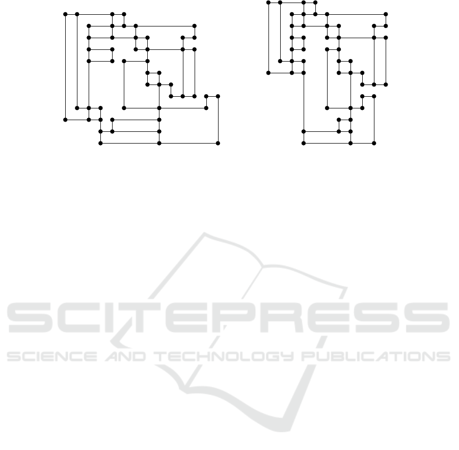
Figure 1: Drawings for the same graph and the same orthogonal shape – with different total edge length.
The complete-extension approach by (Klau and
Mutzel, 1999) was one of the first approaches not
splitting up the compaction problem into two one-
dimensional problems but solving it as a whole, by
formulating it as an integer linear program (ILP).
Eiglsperger and Kaufmann (2002) presented a
linear-time heuristic building up on the basic idea
of (Klau and Mutzel, 1999). Recent research on
the compaction problem was published by (J
¨
unger
et al., 2018), who allow to change the orthogonal
shape of an edge and, under this condition, present
a polynomial-time algorithm. An experimental com-
parison of compaction methods can be found in (Klau
et al., 2001). For an overview of compaction heuris-
tics see e. g. (Eiglsperger et al., 2001).
Another challenge when assigning coordinates to
the vertices is to prevent collisions. First heuristics re-
quired all faces to be rectangular (Tamassia, 1987). If
all faces are rectangular already, the compaction prob-
lem can be solved to optimality in polynomial time
(Di Battista et al., 1999). Otherwise, Tamassia (1987)
inserts artificial edges until all faces are rectangular.
If these artificial edges, however, are randomly ori-
ented horizontally or vertically, an optimal drawing is
no longer guaranteed. Contrariwise, iterating over all
possible ways of inserting artificial edges would take
exponential time.
Figure 1 illustrates how a bad local decision –
when considering only one dimension of the drawing,
or when inserting a ”bad” artificial edge – can affect
the drawing as a whole. The drawing in Figure 1(a)
has a total edge length of 128 units, the drawing in
Figure 1(b) – for the same graph and the same orthog-
onal embedding – has a total edge length of 111 units.
With the turn-regularity approach, Bridgeman
et al. (2000) presented a more sophisticated way
to prevent collisions. They first determine all ver-
tices which could potentially collide, vertices with
so-called kitty corners. Only between these pairs of
vertices artificial edges are inserted in order to sep-
arate these vertices either horizontally or vertically.
Thereby, the turn-regularity approach practically
requires much less artificial edges than rectangular
approaches (Esser, 2014). This becomes important if
the problem is solved as an ILP. Then, less artificial
edges mean less constraints. This avoids inserting
needless place-holders to the drawing.
Nowadays, the turn-regularity approach by
(Bridgeman et al., 2000) and the complete-extension
approach by (Klau and Mutzel, 1999) are the methods
for solving the compaction problem. We will prove
the equivalence of both approaches, more precisely:
A face of an orthogonal representation is turn-regular
(as defined in the first approach) if and only if the
segments bounding this face are separated or can
uniquely be separated (as defined in the second
approach). This is, to our best knowledge, the first
formal proof of equivalence of both approaches.
This paper is organized as follows: Section 2 sum-
marizes the main ideas of the turn-regularity approach
and the complete-extension approach, in Section 3
we prove their equivalence, before we summarize our
results in Section 4.
2 COMPACTION METHODS
In this section we describe both the turn-regularity
approach and the complete-extension approach. We
present basic definitions and theorems from (Bridge-
man et al., 2000) and (Klau and Mutzel, 1999), which
are required for further conclusions. For more details
on graph drawing in general, orthogonal drawings,
and compaction, see e. g. (Di Battista et al., 1999),
(Kaufmann and Wagner, 2001), or (Tamassia, 2013).
IVAPP 2019 - 10th International Conference on Information Visualization Theory and Applications
40

c
1
−1
1 1
1
c
2
(a) Kitty corners.
s
1
s
2
s
7
s
4
s
5
s
6
s
3
s
8
(b) Incomplete shape description.
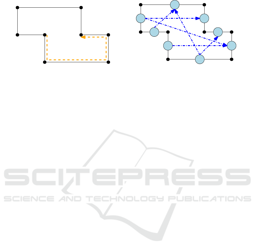
Figure 2: Basic idea of the turn-regularity approach and the complete-extension approach.
Let G = (V, E) be an undirected 4-graph, consist-
ing of a set of n vertices V , and a set of m edges E.
A graph is a 4-graph if it is planar, i. e. it admits a
drawing in the plane without any edge crossings, and
if all vertices have at most four incident edges. Such
a drawing of G in the plane induces a planar embed-
ding and especially specifies the faces in the draw-
ing – multiple internal faces and one external face.
Let H be an orthogonal representation of G. An
orthogonal representation is an extension of a pla-
nar embedding which contains additional information
about the orthogonal shape of the drawing, i. e. infor-
mation about bends along the edges and about the an-
gles between consecutive edges – 90
◦
, 180
◦
, 270
◦
, or
360
◦
angles. Convex (90
◦
) and reflex (270
◦
) corners
are especially important for the turn-regularity ap-
proach. Defining the bends and angles in H implic-
itly specifies which edges are horizontal and which
are vertical.
Hereinafter, w.l.o.g. H is assumed to be simple,
i. e. free of bends, and connected. Existing bends can
beforehand be replaced by artificial vertices. If H is
not connected, each connected component can be pro-
cessed separately.
Let Γ be a planar orthogonal grid drawing of H. In
addition to H, Γ contains information about the coor-
dinates of each vertex on the grid and about the length
of each edge.
Given H, the 2-dimensional compaction problem
is to find a planar orthogonal grid drawing Γ of H with
minimum total edge length. We will focus on this
formulation of the compaction problem. Variations of
this problem, where the area of Γ or the length of the
longest edge is minimized, can be solved with nearly
the same approaches.
2.1 Turn-Regularity Approach
The idea of the turn-regularity approach is to de-
termine all pairs of vertices which could potentially
collide. Unlike for original compaction heuristics
(Tamassia, 1987), the faces are not required to be rect-
angular. The definitions and lemmata within this sub-
section have been adopted from (Bridgeman et al.,
2000).
Definition 1 (Turn). Let f be a face in H. To every
corner c in f a turn is assigned:
turn(c) :=



1, if c is a convex 90
◦
corner,
0, if c is a flat 180
◦
corner,
−1, if c is a reflex 270
◦
corner.
Corners enclosing 360
◦
angles are treated as a pair
of two reflex corners. Bridgeman et al. (2000) have
shown that it is sufficient to replace each 360
◦
vertex
by two artificial 270
◦
vertices connected by an artifi-
cial edge, to subsequently compact the drawing, and
to finally substitute the artificial vertices by the origi-
nal one again.
Thus, in the following we can assume G to be
biconnected, i. e. if an arbitrary vertex was removed
from G, G would still remain connected.
Every reflex corner either is a north-east, south-
east, south-west or north-west corner. If it is clear
which face is considered, we will also speak of north-
east, south-east, south-west, and north-west vertices
which have a respective corner in this face.
Based on turn(c), Bridgeman et al. (2000) defined
the rotation:
Definition 2 (Rotation). Let f be a face in H. The
rotation of an ordered pair of corners (c
i
, c
j
) in f is
defined as
rot(c
i
, c
j
) :=
∑
c∈P
turn(c),
where P is a path along the boundary of f from
c
i
(included) to c
j
(excluded) in counter-clockwise
direction.
For simplifying notation, if it is clear which face
is considered, we also write rot(v
i
, v
j
) for two vertices
v
i
, v
j
with corresponding corners c
i
, c
j
.
Equivalence of Turn-Regularity and Complete Extensions
41

(a) One-dimensional rectangular
approach.
(b) Original turn-regularity
approach with randomly oriented
artificial edges.
(c) Turn-regularity approach
in combination with branch-
and-cut methods.
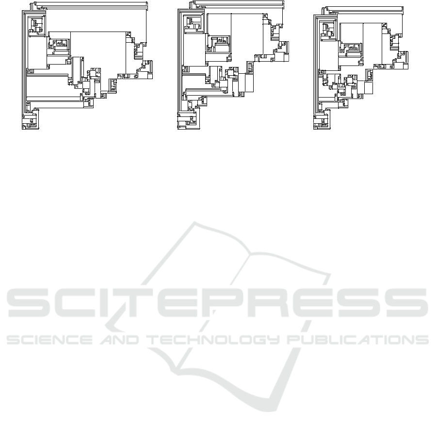
Figure 3: Graph from the ”Rome” dataset compacted by different heuristics with regard to a minimum total edge length.
Lemma 3. Let f be a face in H.
(i) For all corners c
i
in f it holds:
rot(c
i
, c
i
) =

4, if f is an internal face,
−4, if f is the external face.
(ii) For all corners c
i
, c
j
in f the following equiva-
lence holds:
rot(c
i
, c
j
) = 2
⇔ rot(c
j
, c
i
) =

2, if f is an int. face,
−6, if f is the ext. face.
Definition 4 (Kitty Corners, Turn-regular). Let f be
a face in H. Two reflex corners c
i
, c
j
in f are named
kitty corners if rot(c
i
, c
j
) = 2 or rot(c
j
, c
i
) = 2. A
face is turn-regular if it contains no kitty corners.
Figure 2(a) shows two kitty corners c
1
, c
2
within
an internal face. The rotation rot(c
1
, c
2
) (orange,
dashed) sums up to 2.
The kitty corners in H can be determined in a run-
time of O(n) (Bridgeman et al., 2000). If all faces
are turn-regular, an optimal drawing can be computed
in polynomial time by applying minimum-cost flow
techniques as in (Tamassia, 1987).
Otherwise, all non-turn-regular faces are made
turn-regular. Thereby, the turn-regularity approach
defines a heuristic:
1. Determine all non-turn-regular faces.
2. Insert an artificial edge between each pair of kitty
corners.
3. Apply minimum-cost flow techniques to deter-
mine the final length of each edge.
4. Remove the artificial edges.
2.2 Complete-Extension Approach
The complete-extension approach mainly considers
segments, not single edges. A horizontal subsegment
is a set of connected horizontal edges. Note that each
edge is a subsegment itself. A horizontal segment is
a maximally connected horizontal subsegment. This
means that there is no other connected horizontal edge
which could be added to this set. Vertical subseg-
ments and segments are defined analogously.
For a subsegment s, l(s) denotes the vertical seg-
ment containing the leftmost vertex of s; r(s) is the
vertical segment with the rightmost vertex of s, b(s)
and t(s) are the horizontal segments with the bottom-
most and topmost vertex of s. Note that two different
subsegments or edges e
1
, e
2
can have the same left,
right, top or bottom segment, e. g. l(e
1
) = l(e
2
).
The idea of the complete-extension approach by
(Klau and Mutzel, 1999) is to transform the com-
paction problem into a combinatorial problem. For
this purpose so-called shape descriptions are used.
The definitions within this subsection have been
adopted from (Klau and Mutzel, 1999).
Definition 5 (Shape Description, Constraint Graph).
A shape description of the simple orthogonal rep-
resentation H is a tuple σ = hD
h
, D
v
i of two di-
rected so-called constraint graphs D
h
= (S
v
, A
h
) and
D
v
= (S
h
, A
v
) with
A
h
:= {(l(e), r(e)) | e horizontal edge in G},
A
v
:= {(b(e), t(e)) | e vertical edge in G},
and two sets of corresponding vertices S
v
, S
h
.
The arcs in A
h
∪A
v
determine the relative position
of every pair of segments. However, this information
is generally not sufficient to produce an orthogonal
embedding. The shape description might need to be
extended.
IVAPP 2019 - 10th International Conference on Information Visualization Theory and Applications
42

Definition 6 (Separated Segments). A pair of seg-
ments (s
i
, s
j
) ∈ S × S, where S := S
h
∪ S
v
, is called
separated if the shape description contains one of the
four following paths:
1. r(s
i
)
?
−→ l(s
j
) 3. t(s
j
)
?
−→ b(s
i
)
2. r(s
j
)
?
−→ l(s
i
) 4. t(s
i
)
?
−→ b(s
j
)
A shape description is complete if all pairs of seg-
ments are separated.
The notation a −→ b denotes an immediate path
from vertex a to vertex b, while on the path a
?
−→ b
intermediate vertices are allowed.
For two segments (s
i
, s
j
) ∈ S there can exist multi-
ple paths Definition 6, e. g. for two vertical segments
in a rectangular face there exist two paths along the
top way and along the bottom way.
Klau (2001) has shown that it is sufficient to con-
sider only segments within the same face. If any two
segments that share a common face are separated, the
shape description is complete.
Definition 7 (Complete Extension). A complete ex-
tension of a shape description σ = h(S
v
, A
h
), (S
h
, A
v
)i
is a tuple τ = h(S
v
, B
h
), (S
h
, B
v
)i with the following
properties:
(P1) A
h
⊆ B
h
and A
v
⊆ B
v
.
(P2) B
h
and B
v
are acyclic.
(P3) Every non-adjacent pair of segments in G is
separated.
Figure 2(b) shows a shape description (blue, dash-
dotted). The shape description is not complete, as
there is no directed path from segment vertex s
3
to
s
5
and from s
4
to s
6
. If one of the arcs (s
3
, s
5
) or
(s
4
, s
6
) is added, the other pair becomes separated as
well. The shape description then is complete.
From every complete extension an orthogonal
drawing can be constructed which respects all con-
straints of this extension. Thus, the task of com-
pacting an orthogonal grid drawing is equivalent to
finding a complete extension that minimizes the total
edge length. Klau and Mutzel (1999) have formulated
this task as an ILP which can be solved optimally.
If a shape description is complete or uniquely com-
pletable, the compaction problem can be solved opti-
mally in polynomial time (Klau and Mutzel, 1999).
Figure 3 shows a graph from the ”Rome” dataset,
which has been introduced by (Di Battista et al.,
1997). The dataset consists of about 11,000 real-
world graphs and is widely used for benchmarking
graph drawing algorithms.
The drawing in Figure 3(a) (total edge length:
3,276 units) has been compacted by the original
approach by (Tamassia, 1987), which reduces the
problem to two one-dimensional problems and inserts
artificial edges until all faces are rectangular.
For Figure 3(b) (total edge length: 3,154 units) the
turn-regularity approach by (Bridgeman et al., 2000)
has been applied. The original turn-regularity ap-
proach first determines all vertices which could col-
lide, inserts artificial edges between these kitty cor-
ners, but then randomly orients these artificial edges –
either horizontally or vertically. Thus, the approach
generally does not lead to optimal results.
Figure 3(c) (total edge length: 2,882 units) shows
an optimal drawing which has been created by an ”ex-
tended” turn-regularity method. If we do not ori-
ent the artificial edges randomly, but if we apply
branch-and-cut methods to iterate over all feasible
combinations, this leads to an optimal solution. The
complete-extension approach by (Klau and Mutzel,
1999) makes use of the same branch-and-cut tech-
niques. It iterates over all possible combinations to
extend incomplete shape descriptions, and – due to
the equivalence, which we prove in Section 3 – the
complete-extension approach will return an optimal
drawing with the same total edge length. If there ex-
ist multiple optimal solutions, the drawings resulting
from both approaches can differ due to local deci-
sions, but will both have minimum total edge length.
3 EQUIVALENCE
In this section we prove the equivalence of the
turn-regularity approach and the complete-extension
approach. Note that both approaches consider differ-
ent components of a drawing. While turn-regularity is
a definition based on the shape of faces, completeness
is a definition based on segments, more precisely: on
the vertices dual to the segments. However, a segment
is a set of edges, so that a relation between segments
and faces can be established. A segment s is said to
bound a face f if one of the edges in s is on the bound-
ary of f .
When introducing the concept of turn-regularity,
Bridgeman et al. (2000) constructed auxiliary graphs
G
l
, G
r
, H
x
, and H
y
(note that H
x
, H
y
are graphs, not
orthogonal representations).
G
l
is a variation of the original graph G in which
all edges are oriented leftward or upward, in G
r
all
edges are oriented rightward or upward.
Bridgeman et al. (2000) augment G
l
and G
r
by
so-called saturating edges. These saturating edges
are constructed based on a previously defined switch
property of the edges in E. Effectively, the saturat-
ing edges – or the ”saturator” – simply form an acyclic
directed graph with a source vertex s and a target
Equivalence of Turn-Regularity and Complete Extensions
43

(a) Drawing of G
l
(solid lines) and its sat-
urator (dotted lines).
(b) Drawing of G
r
(solid lines) and its
saturator (dashed lines).
(c) Drawing of H
x
.
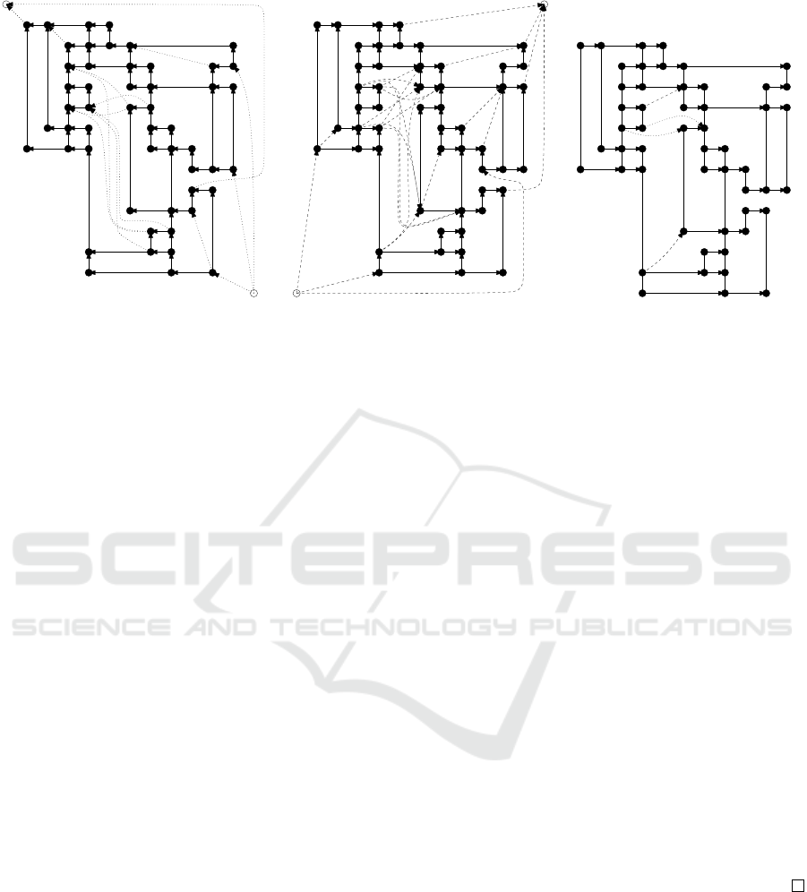
Figure 4: Drawings of the auxiliary graphs G
l
, G
r
, and H
x
.
vertex t. The saturator of G
l
consists of
• additional source and target vertices s and t in the
external face,
• an arc from s to every external south-east vertex,
• an arc from every external north-west vertex to t,
• an arc from every internal north-west vertex to its
opposite convex vertex,
• an arc from the opposite convex vertex to any in-
ternal south-east vertex, and
• the subset of all affected vertices from V .
The saturator of G
r
is defined analogously, with
outgoing arcs from north-east vertices and incoming
arcs towards south-west vertices.
Bridgeman et al. (2000) further introduced max-
imal vertical or horizontal unconstrained chains. A
chain of segments in a face f is said to be uncon-
strained if both its end-vertices have a reflex corner.
Based on G
l
, G
r
, and their saturators, Bridgeman
et al. (2000) constructed two more auxiliary graphs
H
x
, H
y
:
H
x
describes the x-, i. e the left-to-right relation
between the segments in H. H
x
contains all original
edges from E and exactly those saturating edges from
both G
l
and G
r
which are incident to end-vertices of
a maximal unconstrained vertical chain. The orig-
inal vertical edges are kept without orientation, the
original horizontal edges are all oriented from left to
right. The saturating edges in H
x
are all oriented so
that they point from left to right segments (i. e. the
saturating edges from G
l
are reversed). The source
vertex s, the sink vertex t, and all their incident edges
are omitted.
H
y
, which denotes the bottom-to-top relation be-
tween segments, is constructed in a similar way. In
H
y
, the saturating edges are incident to end-vertices of
maximal horizontal unconstrained chains, the vertical
edges are all directed upwards, the horizontal ones are
unoriented.
Figure 4 shows these auxiliary graphs G
l
, G
r
and,
H
x
for the drawing from Figure 1(b). H
y
has not been
illustrated, as it is – apart from the orientation of the
edges – identical with the original graph. There do not
exist horizontal unconstrained chains, so that H
y
does
not contain any saturating edges.
H
x
in this example is not uniquely determined, be-
cause in the non-turn-regular face there exist various
possibilities to add saturating edges. For every maxi-
mal unconstrained vertical chain two incident saturat-
ing edges have been chosen.
Bridgeman et al. (2000) have proven various char-
acteristics of these auxiliary graphs, in particular:
Lemma 8. H
x
and H
y
are uniquely determined if and
only if H is turn-regular.
Proof. See (Bridgeman et al., 2000, p. 71).
We will use this statement when proving the for-
ward direction of the theorem on equivalence.
Bridgeman et al. (2000) later used Lemma 8 to
show that in a turn-regular orthogonal representa-
tion there exist so-called orthogonal relations between
every two vertices (Bridgeman et al., 2000, Theo-
rem 5). This is where the link to the complete-
extension approach is established. A complete exten-
sion of a shape description also means that there is
some unique relation between every two segments.
IVAPP 2019 - 10th International Conference on Information Visualization Theory and Applications
44

Theorem 9. A face f in H is turn-regular if and
only if the segments bounding f are separated or can
uniquely be separated.
Proof. Forward direction: Let f be turn-regular. We
can apply Lemma 8 and conclude that H
x
and H
y
are
uniquely determined. Thus, it needs to be proved that
H
x
and H
y
induce a complete extension.
The horizontal arcs in H
x
are all directed in right
direction, the vertical arcs in H
y
in top direction.
Thus, from the vertical segments we can deduce a set
of segment vertices S
v
. From the horizontal arcs in H
x
we can deduce a set of horizontal left-to-right arcs A
h
connecting these segment vertices. Then, every two
segment vertices in S
v
are connected by a sequence
of arcs from A
h
if there is a corresponding path in
H
x
. Thus, the vertical segments and the horizontal
arcs in H
x
induce a constraint graph D
h
= (S
v
, A
h
). In
the same way, a second constraint graph D
v
= (S
h
, A
v
)
can be deduced from the horizontal segments and the
vertical arcs in H
y
.
Let B
h
contain all arcs from A
h
and all saturating
edges from H
x
. Let B
v
contain all arcs from A
v
and all
saturating edges from H
y
.
It remains to show that τ = h(S
v
, B
h
), (S
h
, B
v
)i is a
complete extension of σ = hD
h
, D
v
i. We will prove
that the three properties from Definition 7 are ful-
filled. As A
h
and A
v
have been augmented by addi-
tional arcs, for (P1) it obviously holds A
h
⊆ B
h
and
A
v
⊆ B
v
.
Regarding (P2), B
h
and B
v
are acyclic by construc-
tion. A
h
only contains left-to-right arcs. The arcs from
B
h
\A
h
do not close any cycles in D
h
as they establish
new left-to-right relations between previously uncon-
nected vertices, i. e. they retain the left-to-right-order
of D
h
. The same argument applies to D
v
and the arcs
from B
v
\ A
v
.
For (P3) we can argue that the saturating edges in
H
x
and H
y
were added at the ends of maximal uncon-
strained chains – which exactly bound non-separated
segments. The end-vertices of a maximal uncon-
strained chain both correspond to reflex corners.
This means that, without the saturating edges, the
unconstrained chain is non-separated from any other
segment. From the other segment vertices in S
h
∪ S
v
there either exist only incoming or only outgoing arcs
to the segment vertices of this unconstrained chain.
Without the saturating edges, a path coming in to the
unconstrained chain and then going out to another
segment, as the paths in Definition 6, could not be
established. The saturating edges, however, allow
exactly these paths, because they are incident with
the end-vertices of unconstrained chains and facili-
tate an additional way towards or away from these
end-vertices. As the saturating edges were added at
the ends of all maximal unconstrained chains, all seg-
ments are separated.
Summarized, we can deduce a complete extension
from H
x
and H
y
. As H
x
and H
y
are uniquely deter-
mined, this complete extension is unique. Thus, for
any turn-regular face f the segments bounding f are
already separated or can uniquely be separated.
Backward direction: One possible way to prove
the backward direction is to give a constructive proof,
to transform an arbitrary complete extension into aux-
iliary representations H
x
, H
y
, and to finally apply
Lemma 8 again. Another way is to translate the lan-
guage of complete extensions into the language of
turn-regularity, and to argue by the rotation. We will
do the latter.
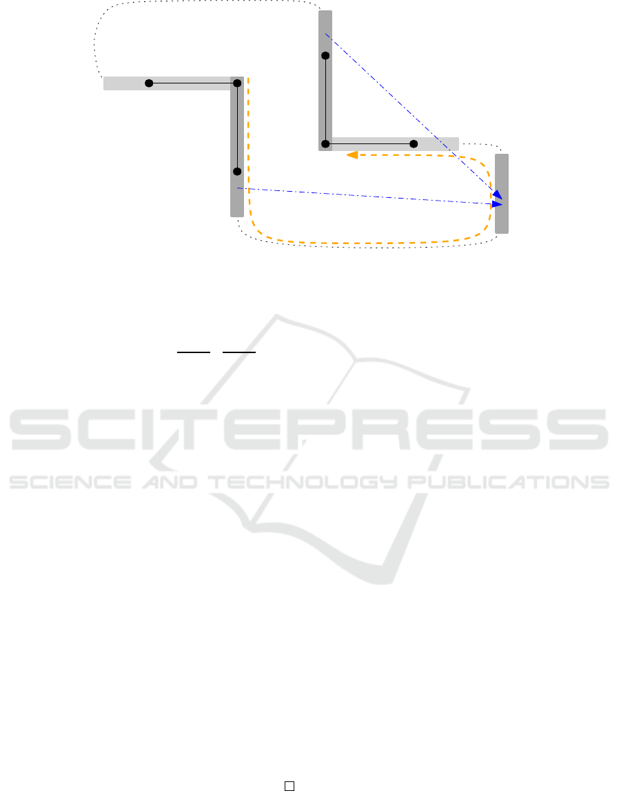
Let f be non-turn-regular, i. e. in f there
exists at least one pair of kitty corners (c
1
, c
2
) with
rot(c
1
, c
2
) = 2. Denote the corresponding vertices by
u
1
, u
2
. Let s
h
1
, s
v
1
be the horizontal and vertical seg-
ment incident to u
1
, and let s
h
2
, s
v
2
analogously be the
incident segments to u
2
. Figure 5 illustrates this set-
ting.
Let first
p
(s) and last
p
(s) be the first and last ver-
tex, respectively, of a segment s on a path p.
Consider the vertical segments s
v
1
, s
v
2
and the
path p = u
1
?
−→ last
p
(s
v
1
)
?
−→ first
p
(s
h
2
)
?
−→ u
2
. In
Figure 5, p is the path along the bottom way.
If f is an internal face, it holds:
rot(u
1
, u
2
) = 2
= − 1 + rot(last
p
(s
v
1
), u
2
)
| {z }
=3
(1)
As the rotation along the subpath last
p
(s
v
1
)
?
−→ u
2
is 3, on this path there must exist at least three convex
corners and at least one other vertical segment s
?
. In
the constraint graph D
h
, the arc between s
v
1
and s
?
and
the arc between s
v
2
, s
?
must both be either incoming
or outgoing due to the rotation.
In Figure 5 both arcs to s
?
are incoming, drawn as
dash-dotted blue arcs.
For the sake of completeness note that if there
are additional vertical segments on the subpath
last
p
(s
v
1
)
?
−→ u
2
, there will not be immediate arcs be-
tween s
v
1
and s
?
or between s
v
2
and s
?
, but a longer
sequence of incoming or outgoing arcs.
Summarized, as both arcs are either incoming or
outgoing, path p from s
v
1
to s
v
2
allows none of the four
connections from Definition 6.
Equivalence of Turn-Regularity and Complete Extensions
45

f
c
2
c
1
u
1
u
2
s
v
2
s
v
1
s
h
1
s
h
2
p
−1
−1
s
?
Figure 5: Illustration of the proof of equivalence.
Following from Lemma 3, it also holds:
rot(u
2
, u
1
) = 2
= − 1 + rot(last
p
(s
v
2
), u
1
)
| {z }
=3
(2)
Thereby, the same conclusion as
above can be shown for the other path
q = u
2
?
−→ last
q
(s
v
2
)
?
−→ first
p
(s
h
1
)
?
−→ u
1
from s
v
2
to s
v
1
. In Figure 5, q is the path along the upper way.
Thus, s
v
1
and s
v
2
are not separated.
If f is the external face, the following two equa-
tions (or vice versa) apply and the same conclusion
can be deduced:
rot(u
1
, u
2
) = 2 = − 1 + rot(last
p
(s
v
1
), u
2
) (3)
rot(u
2
, u
1
) = −6 = − 1 + rot(last
p
(s
v
2
), u
1
) (4)
When considering the horizontal segments s
h
1
, s
h
2
it can be argued in the same way that these segments
are not separated. Thus, neither the vertical segments
s
v
1
, s
v
2
nor the horizontal segments s
h
1
, s
h
2
are separated.
It remains to show that there is no unique way
to complete the shape description. This is because it
holds u
1
= r (s
h
1
) = t(s
v
1
) and u
2
= l(s
h
2
) = b(s
v
2
). This
means that there are two possible ways to complete
shape description, not only one. As soon as – either
in the horizontal or the vertical constraint graph – a
path completing the shape description is chosen, the
respective segments in the other constraint graph will
be separated as well.
Thus, the shape description is not complete and a
complete extension cannot uniquely be chosen.
The forward direction of the proof induces an
algorithm for transferring the turn-regularity formu-
lation into the complete-extension formulation. For
turn-regular orthogonal representations the auxiliary
graphs G
l
, G
r
, their unique saturators, and H
x
, H
y
can be constructed in O (n) time (Bridgeman et al.,
2000, Proof of Theorem 8), (Di Battista and Li-
otta, 1998). Replacing each segment by a segment
vertex and constructing the constraint graphs can
also be done in linear time. This means that the
turn-regularity formulation can be converted into the
complete-extension formulation – when not having to
choose one of many saturators – in O(n) time.
The compaction problem becomes NP-hard if the
orthogonal representation is not turn-regular and one
has to choose from a possibly exponential number
of saturators or, in the complete-extension formula-
tion, from a possibly exponential number of complete
extensions.
4 CONCLUSION
We have shown that the turn-regularity approach by
(Bridgeman et al., 2000) and the complete-extension
approach by (Klau and Mutzel, 1999) are equivalent:
A orthogonal representation is turn-regular if and only
if there exists a unique complete extension. In the
first approach, one must decide how to align new ar-
tificial edges in non-turn-regular faces. In the second
approach, one must decide how to extend incomplete
shape descriptions. Our theorem means that both de-
cisions are equivalent.
Klau and Mutzel (1999) have formulated the com-
paction problem as an ILP. The equivalence of both
approaches suggests that there also exists an ILP for-
mulation for the turn-regularity approach. In (Esser,
2014) a restricted ILP formulation under certain con-
ditions has been presented. We plan to present a gen-
eral ILP formulation.
IVAPP 2019 - 10th International Conference on Information Visualization Theory and Applications
46

Moreover, we want to discuss the meaning of the
equivalence from a practical perspective. Which of
both approaches – in practice – suits best to which use
case? Which approach is more efficient for which
visualization problem?
We further intend to apply compaction techniques
to the area of document processing. Here, a common
issue is to correctly extract tables from documents.
These tables could be interpreted as orthogonal draw-
ings.
ACKNOWLEDGEMENTS
I would like to express my great appreciation to
Christiane Spisla, TU Dortmund University, for many
helpful discussions and constructive suggestions.
REFERENCES
Bannister, M. J. and Eppstein, D. (2012). Hardness of ap-
proximate compaction for nonplanar orthogonal graph
drawings. In GD ’11: Proceedings of the 19th Inter-
national Symposium on Graph Drawing, volume 7034
of Lecture Notes in Computer Science, pages 367–
378. Springer.
Batini, C., Nardelli, E., and Tamassia, R. (1986). A layout
algorithm for data flow diagrams. IEEE Transactions
on Software Engineering, 12(4):538–546.
Batini, C., Talamo, M., and Tamassia, R. (1984). Computer
aided layout of entity relationship diagrams. Journal
of Systems and Software, 4(2-3):163–173.
Bridgeman, S., Di Battista, G., Didimo, W., Liotta, W.,
Tamassia, R., and Vismara, L. (2000). Turn-regularity
and optimal area drawings of orthogonal representa-
tions. Computational Geometry, 16(1):53–93.
Di Battista, G., Eades, P., Tamassia, R., and Tollis, I. (1999).
Graph Drawing: Algorithms for the Visualization of
Graphs. Prentice Hall, Upper Saddle River, USA.
Di Battista, G., Garg, A., and Liotta, G. (1995). An ex-
perimental comparison of three graph drawing algo-
rithms. In SCG ’95: Proceedings of the 11th Annual
Symposium on Computational Geometry, pages 306–
315. ACM.
Di Battista, G., Garg, A., Liotta, G., Tamassia, R., Tassinari,
E., and Vargiu, F. (1997). An experimental compari-
son of four graph drawing algorithms. Computational
Geometry, 7(5-6):303–325.
Di Battista, G. and Liotta, G. (1998). Upward planarity
checking: Faces are more than polygons. In GD ’98:
Proceedings of the 6th International Symposium on
Graph Drawing, pages 72–86. Springer.
Eiglsperger, M. (2003). Automatic Layout of UML Class
Diagrams: A Topology-Shape-Metrics Approach.
PhD thesis, University of T
¨
ubingen, T
¨
ubingen, Ger-
many.
Eiglsperger, M., Fekete, S. P., and Klau, G. W. (2001). Or-
thogonal graph drawing. In Drawing Graphs, pages
121–171. Springer.
Eiglsperger, M. and Kaufmann, M. (2002). Fast compaction
for orthogonal drawings with vertices of prescribed
size. In Graph Drawing, pages 124–138. Springer.
Eiglsperger, M., Kaufmann, M., and Siebenhaller, M.
(2003). A topology-shape-metrics approach for the
automatic layout of UML class diagrams. In SOFT-
VIS ’03: Proceedings of the 2003 ACM Symposium
on Software Visualization, pages 189–198. ACM.
Esser, A. M. (2014). Kompaktierung orthogonaler Zeich-
nungen. Entwicklung und Analyse eines IP-basierten
Algorithmus. Master’s thesis, University of Cologne,
Cologne, Germany.
J
¨
unger, M., Mutzel, P., and Spisla, C. (2018). Orthog-
onal compaction using additional bends. In VISI-
GRAPP/IVAPP ’18: Proceedings of the 13th Inter-
national Joint Conference on Computer Vision, Imag-
ing and Computer Graphics Theory and Applications,
pages 144–155.
Kaufmann, M. and Wagner, D., editors (2001). Drawing
Graphs: Methods and Models, volume 2025 of Lec-
ture Notes in Computer Science. Springer.
Klau, G. W. (2001). A Combinatorial Approach to Orthog-
onal Placement Problems. PhD thesis, Saarland Uni-
versity, Saarbr
¨
ucken, Germany.
Klau, G. W., Klein, K., and Mutzel, P. (2001). An exper-
imental comparison of orthogonal compaction algo-
rithms. In GD ’00: Proceedings of the 8th Interna-
tional Symposium on Graph Drawing, volume 1984
of Lecture Notes in Computer Science, pages 37–51.
Springer.
Klau, G. W. and Mutzel, P. (1999). Optimal compaction
of orthogonal grid drawings. In IPCO ’99: Proceed-
ings of the 7th International Conference on Integer
Programming and Combinatorial Optimization, pages
304–319. Springer.
Lengauer, T. (1990). Combinatorial Algorithms for Inte-
grated Circuit Layout. John Wiley & Sons, Inc.
Patrignani, M. (2001). On the complexity of orthogonal
compaction. Computational Geometry: Theory and
Applications, 19(1):47–67.
Tamassia, R. (1987). On embedding a graph in the grid
with the minimum number of bends. SIAM Journal
on Computing, 16(3):421–444.
Tamassia, R., editor (2013). Handbook on Graph Drawing
and Visualization. Chapman and Hall/CRC.
Tamassia, R., Di Battista, G., and Batini, C. (1988). Au-
tomatic graph drawing and readability of diagrams.
IEEE Transactions on Systems, Man, and Cybernet-
ics, 18(1):61–79.
Equivalence of Turn-Regularity and Complete Extensions
47