Novel View Synthesis using Feature-preserving Depth Map Resampling

Duo Chen, Jie Feng and Bingfeng Zhou

Institute of Computer Science and Technology, Peking University, Beijing, China

Keywords:

Novel View Synthesis, Depth Map, Importance Sampling, Image Projection.

Abstract:

In this paper, we present a new method for synthesizing images of a 3D scene at novel viewpoints, based on a

set of reference images taken in a casual manner. With such an image set as input, our method ﬁrst reconstruct

a sparse 3D point cloud of the scene, and then it is projected to each reference image to get a set of depth

points. Afterwards, an improved error-diffusion sampling method is utilized to generate a sampling point set

in each reference image, which includes the depth points and preserves the image features well. Therefore the

image can be triangulated on the basis of the sampling point set. Then, we propose a distance metric based on

Euclidean distance, color similarity and boundary distribution to propagate depth information from the depth

points to the rest of sampling points, and hence a dense depth map can be generated by interpolation in the

triangle mesh. Given a desired viewpoint, several closest reference viewpoints are selected, and their colored

depth maps are projected to the novel view. Finally, multiple projected images are merged to ﬁll the holes

caused by occusion, and result in a complete novel view. Experimental results demonstrate that our method

can achieve high quality results for outdoor scenes that contain challenging objects.

1 INTRODUCTION

Given a set of reference images of a scene, novel view

synthesis (NVS) methods aim to render the scene at

novel viewpoints. NVS is an important task in com-

puter vision and graphics, and is useful in areas such

as stereo display and virtual reality. Its applications

include 3DTV, Google Street View (Anguelov et al.,

2010), scene roaming and teleconferencing.

NVS methods can be divided into two categories:

small-baseline methods and large-baseline methods,

where “baseline” refers to the translation and rotation

between adjacent viewpoints.

In the case of small-baseline problems, some

methods focus on parameterizing the plenoptic func-

tion with high sampling density. They arrange the

camera positions in well-designed manners and sam-

ple the scene uniformly with reference images. Typ-

ical examples include light ﬁeld (Levoy et al., 1996)

and unstructured lumigraphs (Buehler et al., 2001).

Some other methods (Mahajan et al., 2009; Evers-

Senne and Koch, 2003) were proposed to produce

novel views by interpolating video frames, where ad-

jacent video frames have close viewpoints. Some

methods based on optical ﬂow also belong to the

small-baseline category.

On the other hand, large-baseline NVS is a chal-

lenging, under constrained problem due to the lack of

full 3D knowledge, scale changes and complex oc-

clusions. It is thus necessary to seek additional depth

and geometry information or constraints like photo-

consistency and color-consistency.

For example, Google Street View (Anguelov et al.,

2010) directly acquire depth information with laser

scanners to interpolate large-baseline images. Some

other methods utilize structure-from-motion (SFM)

and multi-view stereo (MVS) to recover sparse 3D

point cloud of the scene and synthesis novel views

based on them. For instance, the rendering algo-

rithm of Chaurasia et al. (Chaurasia et al., 2013) syn-

thesized depth for the poorly constructed regions of

MVS and provides a plausible image-based naviga-

tion. However, their approach is limited by the ca-

pabilities of the oversegmentation, and the very thin

structures in the novel view may be missing.

Recent works also address the problem of large-

baseline NVS by training neural networks in an end-

to-end manner (Flynn et al., 2016). These methods

only require sets of posed images as training dataset,

and are general since they can give good results on

test sets that are considerably different from the train-

ing set. These methods are usually slower than MVS

based methods, and detailed textures in the images are

usually blurred. Moreover, the relationship between

3D objects and their 2D projections has a clear for-

mulation, and requiring neural networks to learn this

Chen, D., Feng, J. and Zhou, B.

Novel View Synthesis using Feature-preserving Depth Map Resampling.

DOI: 10.5220/0007308701930200

In Proceedings of the 14th International Joint Conference on Computer Vision, Imaging and Computer Graphics Theory and Applications (VISIGRAPP 2019), pages 193-200

ISBN: 978-989-758-354-4

193

relationship is inefﬁcient.

The input of our method is a set of photographs

of the scene captured with common commercial cam-

eras, and the camera positions are selected in a ca-

sual manner rather than pre-designed. The position of

novel viewpoints can also be arbitrary, as long as it

is not too far from the existing camera positions. We

ﬁrst reconstruct the scene using SfM and MVS, and

the resulting 3D point cloud is projected to reference

camera positions to get per-view coarse depth maps.

We then apply a feature-preserving sampling and tri-

angulation method to the input images, followed by a

depth propagation step to generate dense depth maps.

Finally, the novel view can be rendered by an image

projection and merging step.

The main contributions of this paper include:

1. We present a method to achieve high quality large-

baseline NVS for challenging scenes. The pro-

posed approach decomposes the problem into four

steps: 1) sparse 3D point cloud reconstruction,

2) importance sampling, 3) depth propagation and

4)image projection and merging.

2. A novel depth propagation algorithm to generate

pixel-wise depth map for reference images based

on resampling and triangulation.

2 RELATED WORK

2.1 Image-based Rendering

Unlike traditional approaches based on geometry

primitives, image-based rendering (IBR) techniques

render novel views based on input image sets. IBR

techniques can be classiﬁed into different categories

according to how much geometry information they

use.

Light ﬁeld rendering (Levoy et al., 1996) and un-

structured lumigraphs (Buehler et al., 2001) are repre-

sentative techniques for rendering with no geometry.

They characterize subsets of the plenoptic function

from high-density discrete samples, and novel views

can be rendered in real time using light ﬁelds or lumi-

graphs. The main limitation of these methods is that

they all require high sampling density, and rendering

novel views far from the existing viewpoints is very

challenging.

View interpolation approaches (Stich et al., 2008;

Mahajan et al., 2009) rely on implicit geometry and

are able to create high-quality transitions between

image sequences or video frames. However, these

methods are only suitable for small-baseline tasks and

hence beyond our consideration.

Some recent works take advantage of the mod-

ern multi-view stereo (MVS) techniques. They uti-

lize the sparse point cloud generated by MVS as

geometric proxies, and project input images to the

novel view. Since these point clouds usually have

poorly constructed regions, Goesele et al. use am-

bient point cloud (Goesele et al., 2010) to represent

unconstructed regions of the scene, and render them

in a non-photorealistic style.

2.2 3D Reconstruction

Structure-from-motion (SfM) has been widely used

for 3D reconstruction from uncontrolled photo collec-

tions. Taken a set of images along with their intrinsic

camera parameters as input, a typical SfM system ex-

tracts feature points in each image and matches them

between image pairs. Then, starting from an initial

two-view reconstruction, the 3D point cloud and per

image external camera matrix is reconstructed by iter-

atively adding new images, triangulating feature point

matches and bundle-adjusting the 3D points and cam-

era poses (Wu, 2013).

Multi-view stereo (MVS) algorithms can recon-

struct reasonable point clouds from multiple pho-

tographs or video clips. The method proposed by Fu-

rukawa and Ponce (Furukawa and Ponce, 2010) takes

multiple calibrated photographs as input, and match

images at both per-pixel and per-view level. The

matching results are improved by optimizing the sur-

face normal within a photo-consistency measure, and

lead to a dense set of patches covering the surfaces of

the object or scene.

However, point clouds reconstructed by MVS are

still relatively sparse, and their distribution is usu-

ally irregular. Although these MVS methods work

well for regular scenes like buildings and sculptures,

objects with complex occlusions or texture-poor sur-

faces are usually poorly constructed or totally miss-

ing, due to the lack of photo-consistency in these re-

gions. Without accurate depth information, MVS-

based NVS approaches are prone to generate unrealis-

tic results, including tearing of occlusion boundaries,

elimination of complete textures or aliasing in such

challenging scenes.

2.3 Depth Synthesis

When depth information is available for every pixel in

reference images, a novel view can be rendered at any

nearby viewpoint by projecting the pixels of the refer-

ence images back to the 3D world coordinate system

and re-projecting them to the novel viewpoint. Thus,

synthesizing dense depth maps from sparse ones is

GRAPP 2019 - 14th International Conference on Computer Graphics Theory and Applications

194

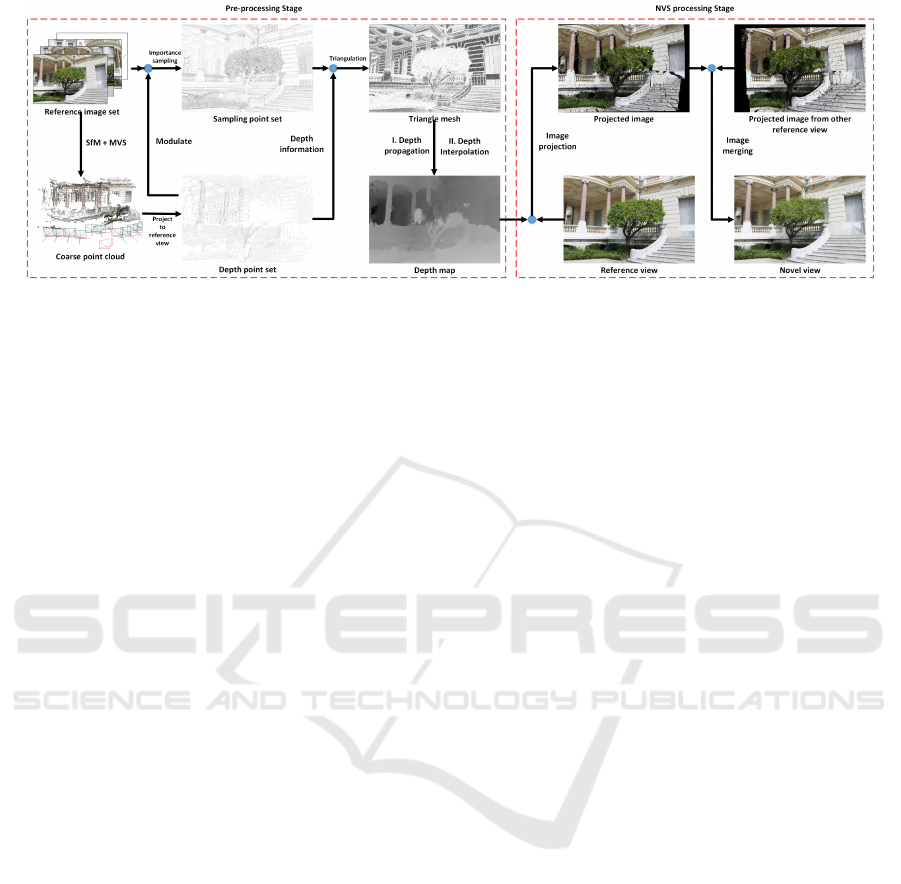
Figure 1: The pipeline of our method.

necessary for our task.

Several works focus on generating dense depth

maps by propagating depth samples to the uncon-

structed pixels of the image. The method proposed

by Lhuillier and Quan (Lhuillier and Quan, 2003) re-

constructs per-view depth maps and introduce a con-

sistent triangulation of depth maps for pairs of views.

Snavely et al. (Snavely et al., 2006) detect intensity

edges using a Canny edge detector, and smoothly in-

terpolate depth maps by placing depth discontinuities

across the edges. Hawe et al. (Hawe et al., 2011)

present an algorithm for dense disparity map recon-

struction from sparse yet reliable disparity measure-

ments. They perform the reconstruction by making

use of the sparsity in wavelet domain based on the the-

ory of compressive sensing. In the work of Chaurasia

et al. (Chaurasia et al., 2013), depth information is

synthesized for poorly reconstructed regions based on

oversegmented superpixels and a graph traversal algo-

rithm. A following shape-preserving warp algorithm

is implemented to achieve image-based navigation.

2.4 Importance Sampling

In this paper, sampling refers to the process of gener-

ating a set of representative pixels from continuous

images, with certain functions controlling the sam-

pling density in different regions. The sampling point

set should preserve the features of input images and

has good distribution property.

In 2001, Ostromoukhov proposed an improved

error-diffusion algorithm by applying variable co-

efﬁcients for different key levels (Ostromoukhov,

2001). Zhou and Fang (Zhou and Fang, 2003) made

furhter improvement using threshold modulation to

remove visual artifacts in the variable-coefﬁcient

error-diffusion algorithm. By controlling the level of

the modulation strength, an optimal result with blue-

noise property can be achieved.

Zhao et al. (Zhao et al., 2013) proposed a high-

efﬁciency image vectorization method based on im-

portance sampling and triangulation. In this method,

a sampling point set is generated on the image plane

according to an important function deﬁned by struc-

ture and color features. Hence this sampling point

set can preserve both edge and internal features in

the image, and possesses good distribution property.

The areas with signiﬁcant features have higher impor-

tance value together with sample point density, and

vise verse. By triangulating the sampling points and

interpolating color inside the triangles, the image can

be easily recovered.

3 OUR APPROACH

3.1 Overview

In this paper, we propose a NVS method based on

feature-preserving depth map resampling and triangu-

lation. The input of our method is a set of reference

images taken from different viewpoints of a scene

(noted as reference image set). For a desired novel

viewpoint, our method is able to generate plausible

novel view image. As shown in Fig.1, the method in-

cludes the following steps:

1) 3D reconstruction and Propagation. First, we

use SfM to extract camera matrices for each input im-

age and reconstruct a very sparse 3D point cloud of

the scene, and then reﬁne it by MVS. The resulting

point cloud is projected to each reference viewpoint,

providing depth information to a set of points (noted

as depth point set) in each reference image.

2) Importance Sampling. Next, an importance func-

tion is deﬁned based on the boundaries and feature

lines in each reference image. Then a sampling point

set is generated according to the importance func-

tion and the depth point set, using an improved error-

diffusion algorithm. The sampling points are triangu-

lated to form a triangle mesh.

Novel View Synthesis using Feature-preserving Depth Map Resampling

195

3) Depth Propation. Afterwards, with a distance

metric which considers Euclidean distance, color sim-

ilarity and color gradient, depth information is propa-

gated from the depth point set to the whole sampling

point set, and depth values are interpolated in each

triangle to reconstruct a dense depth map.

4) Image Projection and Merging. Finally, given

a desired novel viewpoint, several input images are

chosen as reference, and their corresponding col-

ored depth maps are projected onto the novel image

plane. The projected images are merged, and the

holes caused by occlusion are ﬁlled to obtain the ﬁ-

nal image.

Note that in this pipeline, step 1)∼3) belong to

the pre-processing stage, and hence runs ofﬂine only

once. Step 4) is performed online, according to the

desired novel viewpoint.

3.2 3D Reconstruction and Projection

Our input is a set of images {I

|i = 1...n} of a

3D scene taken by commercial cameras at differ-

ent viewpoints, together with their intrinsic matrices

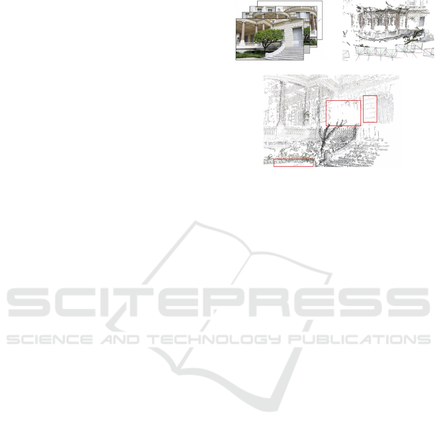
|i = 1...n}. The camera positions are chosen in

a casual manner rather than requiring speciﬁc con-

straints (Fig.2(b)). Instead of reconstructing the com-

plete 3D geometry of the scene, we demonstrate that

a sparse point cloud generated by MVS can provide

enough depth information to generate reliable pixel-

wise depth maps for novel view synthesis.

First, we adopt an SfM method (Wu, 2013) to

extract extrinsic matrices for each camera position,

that is, {R

|i = 1...n} for rotation and {t

|i = 1...n}

for translation. SfM methods can also reconstruct a

sparse point cloud of the scene. On the basis of that,

we further utilize an MVS method (Furukawa and

Ponce, 2010) to reﬁne the 3D point cloud. For the

datasets we use in this paper, the MVS method typ-

ically reconstruct 100k∼200k points from 10 to 30

images with 4M∼6M resolution. The reconstructed

point cloud is irregular for all scenes, regions like

vegetation and walls are often poorly reconstructed

(Fig.2(c)). The depth information for these regions

will be compensated in the following depth synthesis

step.

Then, the 3D point cloud is projected to each ref-

erence viewpoint, producing a set of projected points

with depth information in each input image (Fig.2(c)).

The 3D points and their projections are denoted in ho-

mogeneous notations P = (x,y,z,1) and p = (u,v,1) re-

spectively. The projection is formulated as:

zp = K[R|T]P. (1)

Notice that, some of the projected points should

(a) Reference image set (b) Sparse point cloud

ence view

Figure 2: Input images and reconstructed sparse point

cloud. Note the poorly reconstructed regions shown in (c).

be discarded because of occlusions. While the dis-

tant objects are usually occulded by the near ob-

jects, points belonging to distant objects are hardly

occluded by the near points since they are very sparse,

and therefore wrong depth values will be introduced

to the image.

We tackle this problem by making use of photo-

consistency, i.e., a 3D point P

= (r

) should

have similar color with its corresponding projected

point P

= (r

) for any viewpoint. Therefore,

the projected points whose colors are seriously differ-

ent from their sources will be marked as outliers and

then discarded.

This process also helps to eliminate mistakes in

the sparse point cloud. When the global illumi-

nation does not change radically, the normal Eu-

clidean distance in the RGB or a modiﬁed HSV space

works nearly equally for evaluating color changes

(Hill et al., 1997). Therefore, the color similarity is

measured with the Euclidean distance in RGB color

space throughout this paper.

3.3 Importance Sampling

The depth information produced by SfM / MVS tech-

niques is not sufﬁcient for NVS, for signiﬁcant re-

gions with very sparse or no depth information often

exist. That is because MVS methods reconstruct 3D

points based on feature points matching and photo-

consistency, which will become highly ambiguous for

objects with no or repetitive textures and complex ge-

ometry like self-occlusions. Besides, the number of

reconstructed 3D points is usually less than 5% of the

image pixels, hence the projected points will be sparse

GRAPP 2019 - 14th International Conference on Computer Graphics Theory and Applications

196

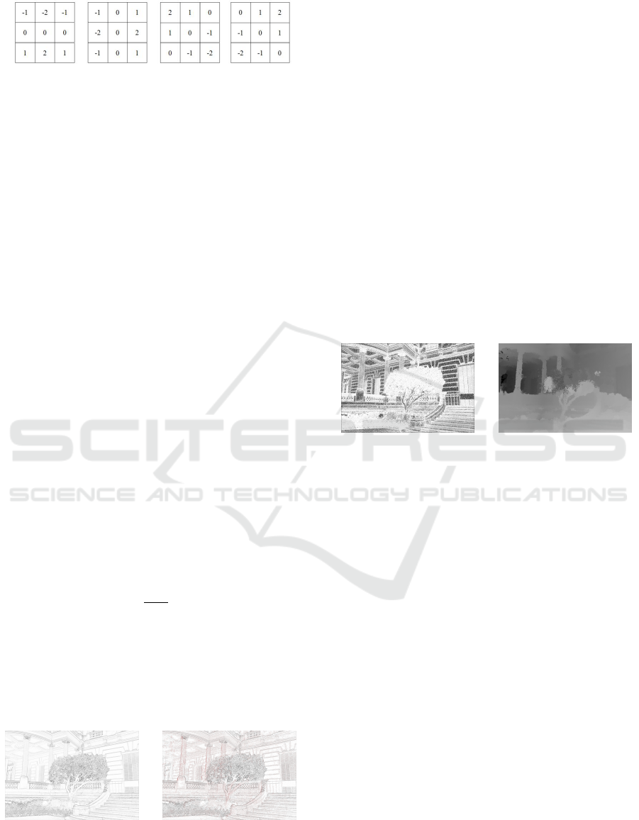
Figure 3: The four templates of the improved Sobel opera-

tor.

and irregular in the depth maps. Directly interpolat-

ing the projected points is prone to create bulky depth

maps with errors near object silhouettes.

In general, depth maps usually consist of large

smooth regions with homogeneous depth values in-

side, and between them existing discontinuities where

depth values change rapidly. Regarding the work of

(Zhao et al., 2013), the large smooth regions can be

represented by a small number of sampling points,

while a large number of sampling points are needed

near the discontinuities.

Although the distribution of smooth regions and

discontinuities in depth maps is previously unknown,

an assumption can be made that discontinuities in the

depth map coincide with the edges in the correspond-

ing reference image. The assumption is not a pre-

cise one, but work well even for the datasets with

quite complex geometry, and the following processes

of sampling and triangulation are robust.

Based on that assumption, we ﬁrst apply an im-

proved Sobel operator (Fig.3) to the reference images

to detect edge features. The improved Sobel operator

contains two more template for diagonal lines, hence

it is able to detect more detailed and accurate features

(shown in Fig.4(a)). Since the resulting gradient val-

ues x are integers ranging from 0 to the maxium gra-

dient over the whole image, we deﬁne an importance

function F to map x from [0,max] to [0,255]:

F(x) = 255[1 − (

max

)

], x ∈ [0, max]. (2)

Here, γ ∈ [0,1] is a constant that controls the im-

portance function. Higher γ will raise the importance

of pixels near the edges, which leads to higher sam-

pling density in these areas, and much lower den-

sity in smooth regions. The distribution of sampling

(a) Egde features (b) The sampling point set

Figure 4: The gradient map (a) preserves the edge features

the reference image. The red points in (b) stand for the

original depth points.

points will be more uniform with lower γ. In our im-

plementation, we set γ to 0.8 to achieve high qual-

ity NVS. Additionally, the importance values of pro-

jected depth points are set to 0 (the highest impor-

tance) to make sure they are sampled.

So far, we obtain an pixel-wise importance map

with importance values ranging from 0 to 255. Then,

an improved error-diffusion sampling method (Zhao

et al., 2013) is performed according to the importance

map to produce the ﬁnal sampling point set (shown in

Fig.4(b)). The number of sampling points is about 10

to 15 % of the total pixels. They have perfect blue-

noise distribution property, and preserve the edge and

internal features in reference images.

We denote the sampling point as P

, which in-

cludes the subset of projected depth points P

. Then,

taking P

as vertices, a triangle mesh is generated by

Delaunay triangluation (shown in Fig.5(a)). The gra-

dient and depth values can be stored in each vertex for

further depth propagation.

(a) Triangle mesh (b) Depth map

Figure 5: (a) Triangle mesh generated by Delaunay trian-

gulating the sampling points. (b) The generated pixel-wise

depth map.

3.4 Depth Propagation

In this step, we propose an efﬁcient and robust ap-

proach to propagate depth information from the pro-

jected depth point set P

to the rest of sampling points

= P

-P

A common observation is that, pixels that are spa-

tially close usually belong to the same object and

hence have similar depth values, unless there is dis-

continuity between them. On another aspect, simi-

lar color in large smooth regions also implies similar

contents and depth values, while color discontinuities

roughly coincide with depth discontinuities.

Thus, we can deﬁne a distance function to eval-

uate the similarity between a pair of pixels, based

on both color and spatial proximity. Euclidean dis-

tance between points P

and P

is calculated in both

RGB color space and reference image coordinate to

describe their similarity. Linear weights k

and k

are

introduce to adjust their inﬂuence.

However, in complex outdoor scenes, neighboring

pixels in reference image may actually belong to

Novel View Synthesis using Feature-preserving Depth Map Resampling

197

distinct objects with very different depths, and in

some situations these pixels also have close colors.

Propagating depth information between these pixels

will destroy the desired discontinuities in the depth

map. We handle this problem by introducing a

penalty term C to limit depth propagation across

object boundaries. The penalty term between P

and

is computed based on the Sobel gradients stored

in the vertices which imply object boundaries in the

image. The ﬁnal form of the distance function is:

D(P

, P

) = {k

[(r

− r

)

+ (g

− g

)

+ (b

− b

)

]

[(u

− u

)

+ (v

− v

)

]}

+C(P

, P

). (3)

C(P

, P

) = argmin

∑

∈Γ

g(P

). (3)

Here Γ represents the set of paths between P

and P

on the triangle mesh. Since larger gradient values im-

ply edges in the image, we take the minimum sum

of the gradients along the paths as the penalty term

C(P

, P

). The shortest path can be calculated by the

Dijkstra shortest path algorithm.

During the closest point searching, a ﬁve-

dimensional kd-tree is built to achieve higher efﬁ-

ciency. The ﬁve dimensions of the kd-nodes include

(u,v) in the image coordinate and (r,g,b) color values.

The distance between kd-nodes is deﬁned similarly to

Eq.3, but without the penalty term. Using the kd-tree,

we ﬁnd the nearest P

for each P

, and calculate the

ﬁnal distance using Eq.3. Hence, for each point in P

its depth value can be propagated from its closest P

After propagating depth information to all the ver-

tices in the triangle mesh, the depth values can be in-

terpolated inside each triangle by a bilinear interpo-

lation and ﬁnally generate a dense pixel-wise depth

map (shown in Fig.5(b)).

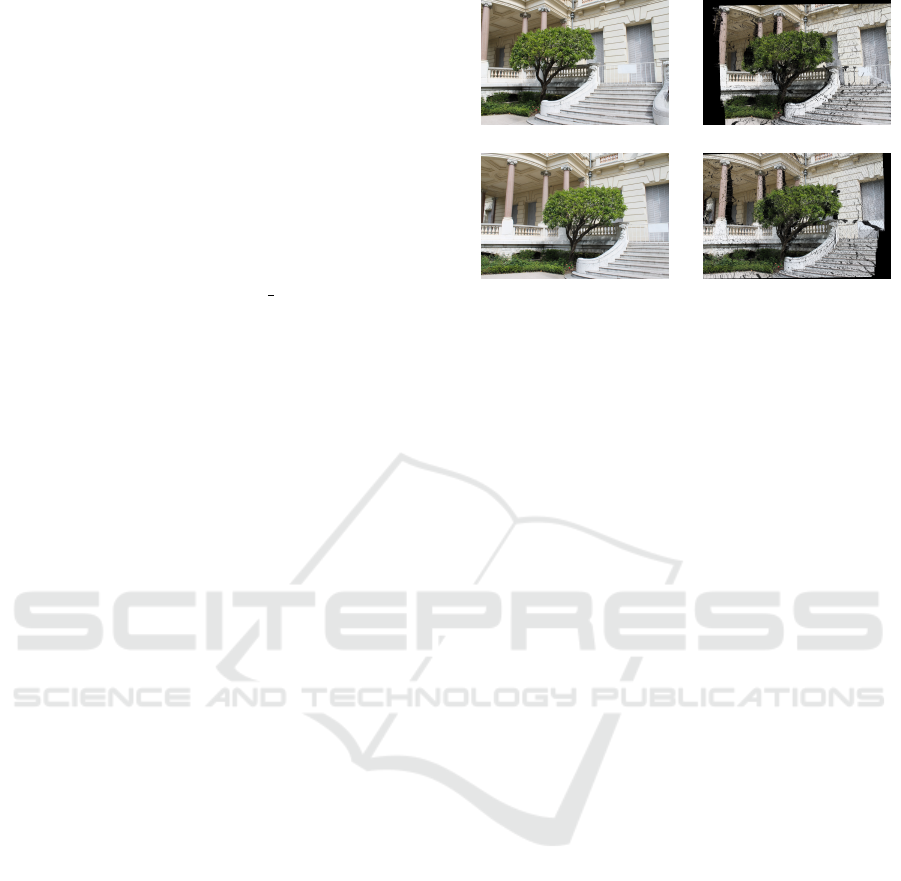
3.5 Image Projection and Merging

After generating dense depth map for each reference

image, a novel view can be interpolated by image pro-

jection. Given a desired novel viewpoint, we ﬁrst se-

lect several input images as reference based on their

camera positions and poses. Then each selected refer-

ence image is projected to the novel viewpoint seper-

ately, exploiting its corresponding depth map (Fig.6).

An intuitive approach for image projection is to

project each pixel in the reference image to the novel

viewpoint discretely. Pixels on the image plane are

back-projected to the world coordinate based on their

depth and the camera matrices, and then projected to

the novel viewpoint. A z-buffer is introduced to han-

dle the occlusions. Regions with no projected pixels

(a) Reference image I

(b) Projected image from I

(d) Projected image from I

Figure 6: Projected images from different reference images.

will be marked as cracks and holes. Holes often ap-

pear near the occusions, while little cracks may ap-

pear everywhere.

In the ﬁnal step of our method, all the projected

image are merged to form a ﬁnal result. For each tar-

get pixel in the novel view, its source pixels will come

from different projected images. Their weights are

assigned according to the depth hints and reference

camera positions. In general, the projected images

whose camera position is closer to the novel view-

point in terms of spatial and angular proximity will be

given higher merging weight. The source pixels may

also come from different objects due to occlusions,

hence we increase the merging weight of the source

pixels with lower depth values. Besides, cracks and

holes in the projected image will share no merging

weight. After the merging step, the majority of holes

and cracks could be ﬁlled, and the remaining ones can

be further eliminated using median ﬁltering.

4 EXPERIMENTAL RESULTS

We test our NVS method on several datasets from

(Chaurasia et al., 2013), including scenes with se-

vere occlusions and challenging objects. In order to

evaluate the effectiveness our method, we take one

image in each dataset as ground truth and synthesize

novel view at the same position. All the algorithms

are implemented on a laptop with Intel Core i5-7300

2.50GHz CPU. Note that in our method, all the steps

except image projection and merging run only once.

The time costs of all the steps for different datasets

and resolution are listed in Table1.

In Fig.7, our synthesizing results are compared to

the ground truth. Result images on University and

Museum2 datasets are shown in Fig.8 together with

corresponding ground truth. In Fig.9 we show the

GRAPP 2019 - 14th International Conference on Computer Graphics Theory and Applications

198

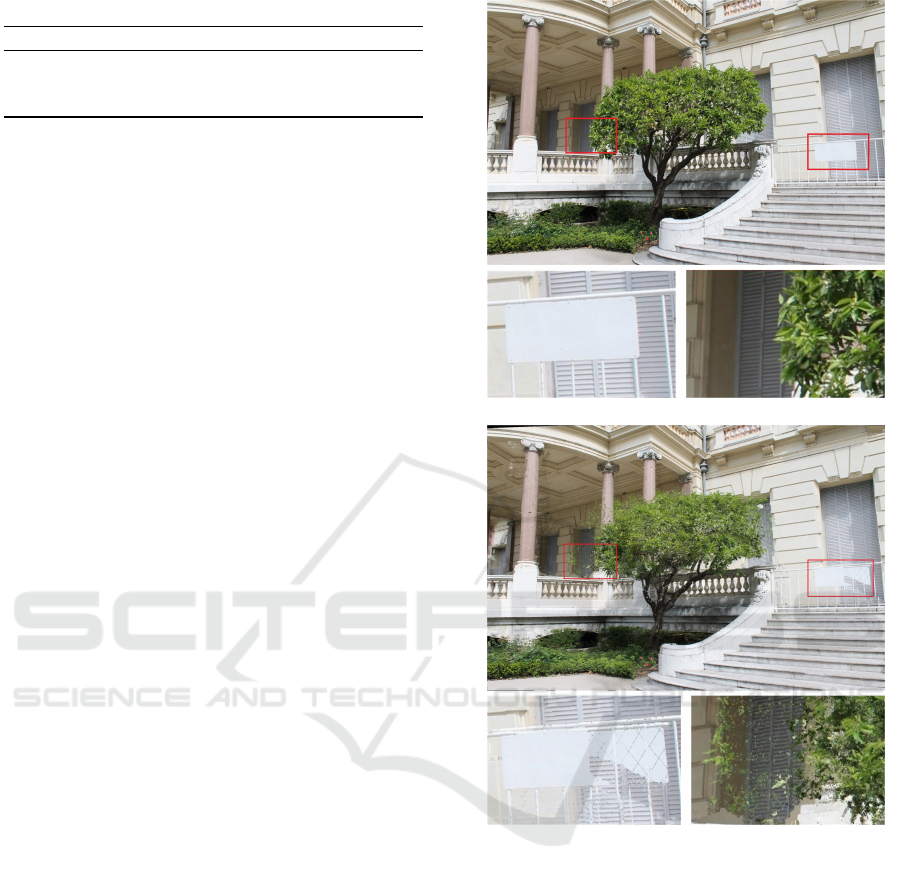
Table 1: Running time for all the steps.

Dataset Resolution Step 1(s) Step 2(s) Step 3(s) Step 4(s)

Museum1 2256*1504 294 78 150 36

Museum1 1200*900 231 27 10 12

Museum2 2256*1504 363 87 103 35

University 1728*1152 168 46 15 19

depth map generated using different set of kd-tree pa-

rameters, and demonstrate their effect on the follow-

ing projection step.

Fig.7 illustrates that our method can produce plau-

sible result image for challenging scenes containing

vegetations and complex occlusions. However, neigh-

boring objects with similar color may have very dif-

ferent depth, e.g. white railing in foreground and

white window blind in background (lower right in

Fig.7(b)). This will lead to misalignment in the depth

synthesis step and result in distortions in the result im-

age. Since all the pixels are projected to novel view-

points discretely, our image projection and merging

step cannot ensure the completeness of image tex-

utres. The broken textures will appear as fragments

in result image (lower left in Fig.7(b)), and decrease

the image quality seriously.

and k

are the two parameters controlling the

distance function Eq.3 in triangle mesh, and they

stand for the weight of color and spatial proximity

respectively. As shown in Fig.9, smaller k

leads to

bulky depth map, and the object boundaries appear

irregular. As the value of k

increases, depth map be-

comes smoother or even be overﬁtted to the image

texture.

Fig.8 demonstrate that our method can render re-

gions with complex texture properly (e.g. words

on warning board in Fig.8(b) and the billboard in

Fig.8(d)). Objects involving severe occlusion (the

huge pillar in Fig.8(b)) can also be well rendered us-

ing a simple z-buffer. Besides, the black region on the

left edge of Fig.8(b) means that pixels in this area are

absent in all other reference images.

5 CONCLUSIONS

In this paper, we propose a novel method for syn-

thesizing novel views from a set of reference im-

ages taken in a casual manner. Our method has a

pre-processing stage consisting of 3D reconstruciton,

importance sampling and depth propagation steps to

generate pixel-dense depth maps for each reference

view, and a projection and merging step for rendering.

We show the efﬁciency and robusness of our method

on some challenging outdoor scenes containing vege-

tations and complex geometry.

The main limitaion of our method is the rendering

(a) Ground truth

(b) Result image

Figure 7: Novel view synthesis result comparison for Mu-

seum1 dataset.

speed. We will implement the image projection and

merging step on GPU for acceleration, and investigate

new rendering algorithms.

Our future work also includes making more use

of photo-consistency. Although the sparse point

cloud generated by MVS is supposed to be photo-

consistent, in some regions of our synthesized depth

maps, this desired property will be lost. We would

like to reﬁne our depth maps by applying photo-

consistency, which will help revising the wrong depth

values.

Novel View Synthesis using Feature-preserving Depth Map Resampling

199

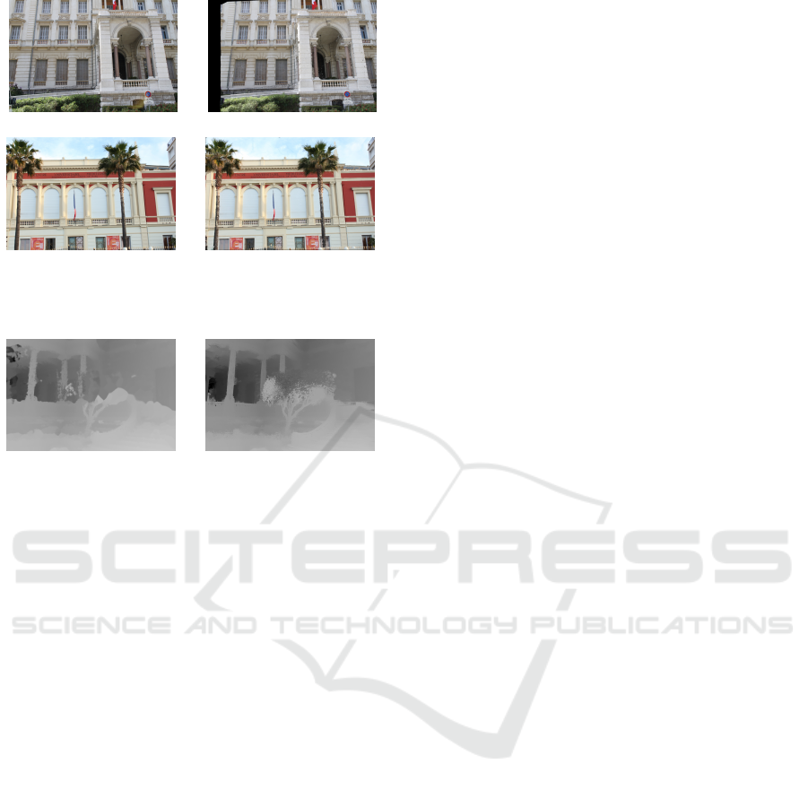
(a) Ground truth (b) Result image

Figure 8: Result comparison for University (a)(b) and Mu-

seum2 (c)(d) dataset.

(a) Depth map 1 (b) Depth map 2

Figure 9: Depth maps generated using different kd-tree pa-

rameters. (a) the depth map with k

= 0.5 k

, (b) depth map

with k

= 10 k

ACKNOWLEDGEMENTS

This work was supported by National Natural Sci-

ence Foundation of China (NSFC) [grant number

61602012].

REFERENCES

Anguelov, D., Dulong, C., Filip, D., Frueh, C., Lafon,

S., Lyon, R., Ogale, A., Vincent, L., and Weaver, J.

(2010). Google street view: Capturing the world at

street level. Computer, 43(6):32–38.

Buehler, C., Bosse, M., Mcmillan, L., Gortler, S., and Co-

hen, M. (2001). Unstructured lumigraph rendering.

In Conference on Computer Graphics and Interactive

Techniques, pages 425–432.

Chaurasia, G., Duchene, S., Sorkine-Hornung, O., and

Drettakis, G. (2013). Depth synthesis and local warps

for plausible image-based navigation. Acm Transac-

tions on Graphics, 32(3):1–12.

Evers-Senne, J. F. and Koch, R. (2003). Image based inter-

active rendering with view dependent geometry. Com-

puter Graphics Forum, 22(3):573582.

Flynn, J., Neulander, I., Philbin, J., and Snavely, N. (2016).

Deep stereo: Learning to predict new views from the

world’s imagery. In Computer Vision and Pattern

Recognition, pages 5515–5524.

Furukawa, Y. and Ponce, J. (2010). Accurate, dense, and ro-

bust multiview stereopsis. IEEE Transactions on Pat-

tern Analysis and Machine Intelligence, 32(8):1362–

1376.

Goesele, M., Ackermann, J., Fuhrmann, S., Haubold, C.,

Klowsky, R., Steedly, D., and Szeliski, R. (2010). Am-

bient point clouds for view interpolation. Acm Trans-

actions on Graphics, 29(4):1–6.

Hawe, S., Kleinsteuber, M., and Diepold, K. (2011).

Dense disparity maps from sparse disparity measure-

ments. In International Conference on Computer Vi-

sion, pages 2126–2133.

Hill, B., Roger, T., and Vorhagen, F. W. (1997). Compar-

ative analysis of the quantization of color spaces on

the basis of the cielab color-difference formula. Acm

Transactions on Graphics, 16(2):109–154.

Levoy, Marc, and Hanrahan (1996). Light ﬁeld rendering.

Computer Graphics.

Lhuillier, M. and Quan, L. (2003). Image-based rendering

by joint view triangulation. IEEE Transactions on Cir-

cuits and Systems for Video Technology, 13(11):1051–

1063.

Mahajan, D., Huang, F. C., Matusik, W., Ramamoorthi, R.,

and Belhumeur, P. (2009). Moving gradients: a path-

based method for plausible image interpolation. In

ACM SIGGRAPH, page 42.

Ostromoukhov, V. (2001). A simple and efﬁcient error-

diffusion algorithm. Proc Siggraph, pages 567–572.

Snavely, N., Seitz, S. M., and Szeliski, R. (2006). Photo

tourism: Exploring photo collections in 3d. Acm

Transactions on Graphics, 25(3):pgs. 835–846.

Stich, T., Linz, C., Wallraven, C., Cunningham, D., and

Magnor, M. (2008). Perception-motivated interpola-

tion of image sequences. pages 97–106.

Wu, C. (2013). Towards linear-time incremental structure

from motion. In International Conference on 3d Vi-

sion, pages 127–134.

Zhao, J., Feng, J., and Zhou, B. (2013). Image vectorization

using blue-noise sampling. Proceedings of SPIE - The

International Society for Optical Engineering, 8664.

Zhou, B. and Fang, X. (2003). Improving mid-tone qual-

ity of variable-coefﬁcient error diffusion using thresh-

old modulation. Acm Transactions on Graphics,

22(3):437–444.

GRAPP 2019 - 14th International Conference on Computer Graphics Theory and Applications

200