Structural Change Detection by Direct 3D Model Comparison

Marco Fanfani and Carlo Colombo

Department of Information Engineering (DINFO), University of Florence, Via S. Marta 3, 50139, Florence, Italy

Keywords:

Change Detection, 3D Reconstruction, Structure from Motion.

Abstract:

Tracking the structural evolution of a site has important ﬁelds of application, ranging from documenting the

excavation progress during an archaeological campaign, to hydro-geological monitoring. In this paper, we

propose a simple yet effective method that exploits vision-based reconstructed 3D models of a time-changing

environment to automatically detect any geometric changes in it. Changes are localized by direct comparison

of time-separated 3D point clouds according to a majority voting scheme based on three criteria that compare

density, shape and distribution of 3D points. As a by-product, a 4D (space + time) map of the scene can also

be generated and visualized. Experimental results obtained with two distinct scenarios (object removal and

object displacement) provide both a qualitative and quantitative insight into method accuracy.

1 INTRODUCTION

Monitoring the evolution over time of a three-

dimensional environment can play a key role in se-

veral application ﬁelds. For example, during an

archaeological campaign it is often required to re-

cord the excavation progress on a regular basis. Si-

milarly, tracking of changes can be useful to con-

trast vandalism in a cultural heritage site, to prevent

natural damages and reduce hydro-geological risks,

and for building construction planning and manage-

ment (Mani et al., 2009).

A simple strategy to change tracking requires that

photos or videos of the scene are acquired and in-

spected regularly. However, a manual checking of

all the produced data would be time consuming and

prone to human errors. To solve this task in a fully

automatic way, 2D and 3D change detection methods

based on computer vision can be employed.

Vision-based change detection is a broad topic

that includes very different methods. They can be

distinguished by the used input data—pairs of ima-

ges, videos, image collections or 3D data—and by

their application scenarios, that can require different

levels of accuracy. In any case, all methods have

to consider some sort of registration to align the in-

put data before detecting the changes. Through the

years, several methods have been proposed (Radke

et al., 2005). The ﬁrst approaches were based on

bi-dimensional data, and used to work with pairs of

images acquired at different times. In order to de-

tect actual scene changes, geometric (Brown, 1992)

and radiometric (Dai and Khorram, 1998; Toth et al.,

2000) registration of images were implemented to

avoid detection of unrelevant changes due to differen-

ces in point of view or lighting conditions. Video-

surveillance applications (Collins et al., 2000) were

also considered: In this case a video of a scene acqui-

red from a single point of view is available, and

change detection is obtained by modelling the back-

ground (Toyama et al., 1999; Cavallaro and Ebrahimi,

2001)—typically using mixture-of-Gaussian models.

Successively, solutions exploiting three-dimensional

information were introduced, in order to obtain bet-

ter geometric registration and mitigate problems rela-

ted to illumination changes. In (Pollard and Mundy,

2007), the authors try to learn a world model as a

3D voxel map by updating it continuously when new

images are available—a sort of background model-

ling in 3D. Then change detection is performed by

checking if the new image is congruent with the le-

arned model. However, camera poses are supposed

to be known and lighting conditions are kept almost

constant. Other methods exploit instead a 3D model

pre-computed from image collections (Taneja et al.,

2011; Palazzolo and Stachniss, 2017) or depth esti-

mates (Sakurada et al., 2013) of the scene so as to

detect structural changes in new images. After regis-

tering the new image sequence on the old 3D model—

using feature matching and camera resectioning (Ta-

neja et al., 2011; Sakurada et al., 2013) or exploiting

also GPS and inertial measurements (Palazzolo and

760

Fanfani, M. and Colombo, C.

Structural Change Detection by Direct 3D Model Comparison.

DOI: 10.5220/0007260607600767

In Proceedings of the 14th International Joint Conference on Computer Vision, Imaging and Computer Graphics Theory and Applications (VISIGRAPP 2019), pages 760-767

ISBN: 978-989-758-354-4

Stachniss, 2017)—change detection is obtained by re-

projecting a novel image onto the previous views by

exploiting the 3D model, so as to highlight possible

2D misalignments, indicating a change in 3D. Howe-

ver, these solutions ﬁnd not only structural changes

but also changes due to moving objects (i.e. cars, pe-

destrians, etc.) that can appear in the new sequence:

in order to discard such nuisances, object recogni-

tion methods have been trained and used to select

changed areas to be discarded (Taneja et al., 2011).

In (Taneja et al., 2013), a similar solution is adop-

ted, using instead a cadastral 3D model and panora-

mic images. Differently, in (Qin and Gruen, 2014)

the reference 3D point cloud is obtained with an accu-

rate yet expensive laser scanning technology; chan-

ges are then detected in images captured at later ti-

mes by re-projection. Note that, in order to register

the laser-based point cloud with the images, control

points have to be selected manually. More recently,

even deep network have been used to tackle change

detection (Alcantarilla et al., 2016) using as input re-

gistered images from the old and new sequences.

Differently from the state-of-the-art, in this pa-

per we propose a simple yet effective solution ba-

sed on the analysis of 3D reconstructions computed

from image collections acquired at different times. In

this way, our method focuses on detecting structural

changes and avoids problem related to difference in

illumination, since it exploits only geometric infor-

mation from the scene. Moreover, 3D reconstruction

methods such as Structure from Motion (SfM) (Sze-

liski, 2010), Simultaneous Localization and Mapping

(SLAM) (Fanfani et al., 2013) or Visual Odome-

try (Fanfani et al., 2016) build 3D models of ﬁxed

structures only, thus automatically discarding any mo-

ving elements in the scene. By detecting differences

in the 3D models, the system is able to produce an

output 3D map that outlines the changed areas. Our

change detection algorithm is fully automatic and is

composed by two main steps: (i) initially, a rigid re-

gistration at six degrees of freedom has to be esti-

mated in order to align the temporally ordered 3D

maps; (ii) then, the actual change detection is per-

formed by comparing the local 3D structures of cor-

responding areas. The detected changes can also be

transported onto the input photos/videos to highlight

the image areas with altered structures. It is worth

noting that our method is easy to implement and can

be sided with any SfM software—as for example Vi-

sualSFM (Wu, 2013) or COLMAP (Sch

onberger and

Frahm, 2016), both freely available—to let even non

expert users build their own change detection system.

2 METHOD DESCRIPTION

Let I

and I

be two image collections of the same

scene acquired at different times t

and t

. At ﬁrst, our

method exploits SfM approaches to obtain estimates

for the intrinsic and extrinsic camera parameters and

a sparse 3D point cloud representing the scene, for

both I

and I

. We also retain all the corresponden-

ces that link 2D points in the images with 3D points

in the model. Then, the initial point clouds is enri-

ched with region growing approaches (Furukawa and

Ponce, 2010) to obtain more dense 3D data. Note that

camera positions and both the sparse and dense mo-

dels obtained from I

and I

are expressed in two in-

dependent and arbitrary coordinate systems, since no

particular calibration is used to register the two col-

lections.

Hereafter we present the two main steps of the

change detection method: (i) to estimate the rigid

transformation that maps the model of I

onto that of

, implicitly exploiting the common and ﬁxed struc-

tures in the area, (ii) to detect possible changes in the

scene by comparing the registered 3D models.

2.1 Photometric Rigid Registration

Since 3D models obtained through automatic re-

construction methods typically include wrongly es-

timated points, before using a global registration

approach—such as the Iterative Closest Point (ICP)

algorithm (Besl and McKay, 1992)—our system ex-

ploits the computed correspondences among image

(2D) and model (3D) points, to obtain an initial esti-

mate of the rigid transformation between the two 3D

reconstructions.

Once computed the sparse reconstructions S

and

, from I

and I

respectively, for each 3D point we

can retrieve a list of 2D projections and, additionally,

for each 2D projection a descriptor vector based on

the photometric appearance of its neighbourhood is

also recovered. Exploiting this information, we can

establish correspondences among images in I

and I

as follows. Each image in I

is compared against all

images in I

and putative matches are found using the

descriptor vectors previously computed. More in de-

tail, let f

= {m

, , m

} be the set of N 2D features

in image I

∈ I

that have an associated 3D point, and

= {m

, , m

} the set relative to I

∈ I

. For each

2D point in f

we compute its distance w.r.t. all points

in f

by comparing their associated descriptor vec-

tors. Then, starting from the minimum distance ma-

tch, every point in f

is put in correspondence with a

point in f

Structural Change Detection by Direct 3D Model Comparison

761

Since we know the relation between 2D and 3D

points in S

and S

, once obtained the matches bet-

ween the 2D point sets, we can promote these rela-

tionships to 3D: Suppose the point m

∈ f

is rela-

ted to the 3D vertex X

∈ S

, and similarly the point

∈ f

is related to the 3D vertex X

∈ S

, then if

matches m

, X

and X

can be put in correspon-

dence with each other. In this way, all the 2D matches

found can be transformed into correspondences of 3D

points.

3D correspondences obtained by comparing all

images in I

with every image in I

are accumulated

into a matrix Q. Since erroneous matches are possi-

ble, inconsistent correspondences could be present in

Q. To extract a consistent matching set

Q, we count

the occurrences of a match in Q (note that, since a 3D

point can be the pre-image of several 2D points, by

comparing all images, we can ﬁnd multiple occurren-

ces). Starting from the most frequent, a match is se-

lected and copied into

Q, then all matches in Q that in-

clude points already present in

Q are removed. Once

completed this analysis, and emptied Q,

Q will de-

ﬁne a consistent 3D matching set without repetitions

or ambiguous correspondences.

An initial rigid transformation between S

and S

is then computed using (Horn, 1987), by exploiting

the 3D matches in

Q. Since wrong correspondences

could still be present in

Q, we include a RANSAC fra-

mework by randomly selecting three correspondences

per iteration. Inliers and outliers are found by obser-

ving the cross re-projection error. For example, if

1,0

is a candidate transformation that maps S

onto

, the system evaluates re-projection errors between

the transformed 3D

= T

1,0

) and the 2D points

of the images in I

and vice-versa, using 3D points

from

= T

−1

1,0

) and 2D points from I

. The best

transformation T

∗

1,0

is estimated using the largest in-

lier set. Now, let D

and D

be the dense reconstructi-

ons obtained respectively from S

and S

using a re-

gion growing approach. As ﬁnal step, our system runs

an ICP algorithm using as input D

and

= T

∗

1,0

to reﬁne the registration.

Note also that, once the registration is completed,

the 3D maps can be easily overlapped so as to visually

observe the environment evolution and produce a 4D

map (space + time).

2.2 Structural Change Detection

Once the 3D models are registered, surface normal

vectors are computed for both D

and D

: for each

vertex, a local plane is estimated using neighbouring

3D points, then the plane normal is associated to the

3D vertex.

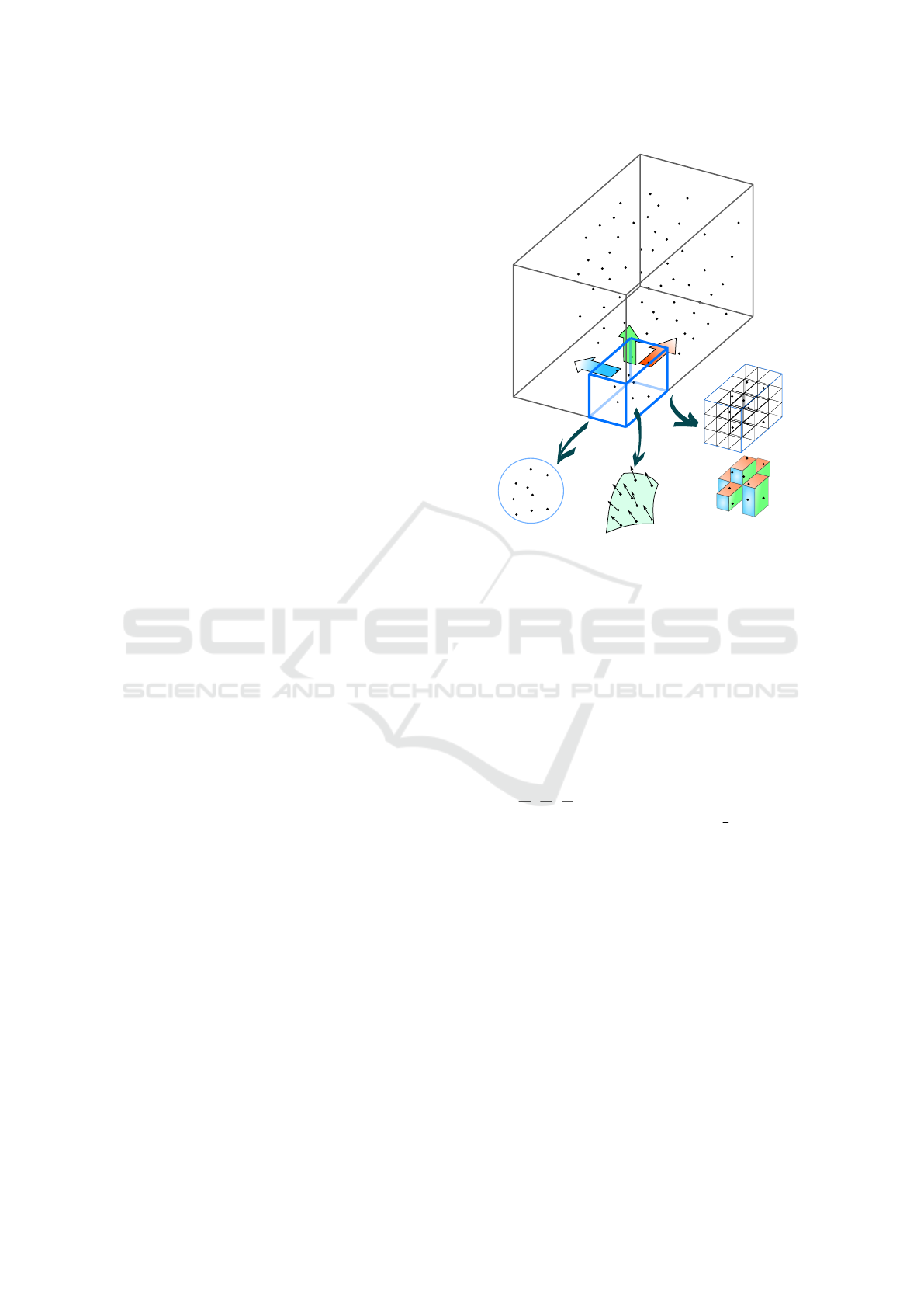
Quantity

Orientation

Occupancy

Figure 1: Graphical representation of our change detection

method. Top: the volume B and the voxel V that shifts

across the point cloud. Bottom: the three criteria used to

detect changes: Quantity, that takes into account the num-

ber of 3D points enclosed in V , Orientation, that is rela-

ted to the local 3D shape, and Occupancy,that describes the

spatial point distribution in V.

Change detection works by shifting a 3D box

over the whole space occupied by the densely recon-

structed model. A bounding volume B is created so

as to include all points in D

and D

, then a voxel V

is deﬁned whose dimensions (V

, V

) are respecti-

vely (

). V is progressively shifted to cover

the entire B volume with an overlap of

between ad-

jacent voxels. Corresponding voxels in D

and D

are

then compared by evaluating the enclosed 3D points

with three criteria named Quantity, Orientation and

Occupancy (see Fig. 1).

Quantity Criterion. The quantity criterion compa-

res the effective number of 3D points in V for D

and

. If their difference is greater than a threshold α,

the criterion is satisﬁed. Note that, even if counting

the 3D points easily provides hints about a possible

change, this evaluation can be misleading since D

and D

could have different densities—i.e. the same

area, without changes, can be reconstructed with ﬁner

or rougher details, mostly depending on the number

and the resolution of the images used to build the 3D

model.

VISAPP 2019 - 14th International Conference on Computer Vision Theory and Applications

762

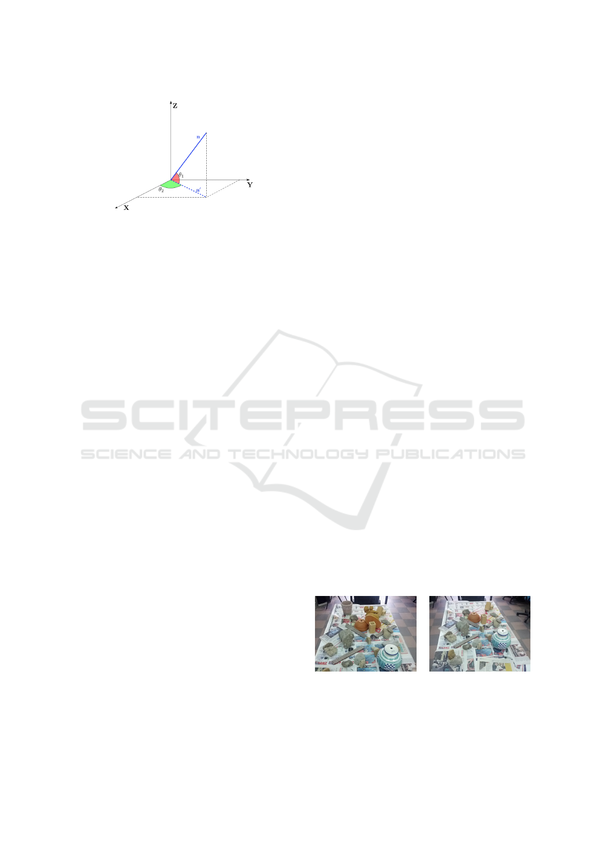
Figure 2: The angles used to describe normal vector orien-

tation.

Orientation Criterion. To evaluate local shape si-

milarity, the normal vectors of points included in V ,

both for D

and D

, are used. For each normal n we

deﬁne its orientation by computing the angles θ

, be-

tween n and its projection n

onto the XY -plane, and

, between n

and the X axis (see Fig. 2). Quantized

values of both θ

and θ

for all considered 3D points

are accumulated in a 2D histogram to obtain a des-

criptor of the surfaces enclosed in V, both for D

and

. These descriptors are then vectorized by concate-

nation of their columns, and the Euclidean distance

(spanning the dimensions of the histogram bins) is

employed to evaluate their similarity. If the distance

is greater than a threshold β, the orientation criterion

is satisﬁed. Note that the reliability of this criterion is

compromised if too few 3D points (and normal vec-

tors) are included in V ; hence, we consider this crite-

rion only if the number of 3D points in V is greater

than a threshold value µ for both D

and D

Occupancy Criterion. This last criterion is used to

evaluate the overall spatial distribution of points in V .

The voxel V is partitioned into 3

= 27 sub-voxels.

Each sub-voxel is labeled as “active” if at least one

3D point falls into it; again, for both D

and D

we construct this binary occupancy descriptor. If

more than γ sub-voxels have different labels, then the

occupancy criterion is satisﬁed.

If at least two out of these three criteria are satis-

ﬁed, a token is given to all points enclosed in V, both

for D

and D

. Once V has been shifted so as to cover

the entire B volume, a 3D heat-map can be produced

by considering the number of tokens received by each

3D point in B, referred to as change score.

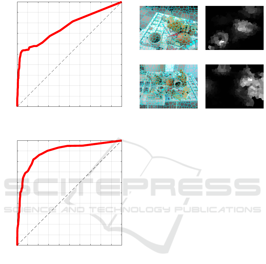
2.3 2D Change Map Construction

Since it could be difﬁcult to appreciate the change de-

tection accuracy just by looking at the 3D heat-map

(examples of which are in Fig. 6), results will be pre-

sented in terms of a 2D change map. This is con-

structed by projecting the 3D points onto one of the

input images, and assigning a colour to each projected

point related to the local change score. Although bet-

ter than the heat-map, the 2D map thus obtained is

sparse and usually presents strong discontinuities (see

e.g. Fig. 8). This is mainly due to the use of a sparse

point cloud as 3D representation. Since any surface

information is missing, we cannot account for cor-

rect visibility of 3D points during the projection. As

a consequence, some points falling on scene objects

actually belong to the background plane.

In order to improve the 2D map, we split the

input image into superpixels, using the SLIC met-

hod (Achanta et al., 2012) (see Fig. 10a and 10c) and

then, for each superpixel, we assign, to all the pixels

in it, the mean change score value of the 3D points

that project onto the superpixel. The resulting 2D

change maps is denser and smoother w.r.t. the pre-

vious one (see Fig. 10b and 10d).

3 EXPERIMENTAL EVALUATION

To evaluate the accuracy of the proposed method we

ran two different tests with datasets recorded in our

laboratory. In the ﬁrst test (”Object removal”), we

built a scene simulating an archaeological site where

several artefacts are scattered over the ground plane

and we acquired a ﬁrst collection of images I

. Then

we removed two objects (the statue and the jar) and

acquired a second collection I

(see Fig. 3).

For the second test (”Object insertion and displa-

cement”), using a similar scene with objects positi-

oned according to a different setup, we recorded the

collection I

. The original setup was then changed

by inserting two cylindrical cans on the left side, by

laying down the statue on the right side and by dis-

placing in a new position the jar, the rocks, and the

bricks. A new collection I

was then acquired (see

Fig. 4).

(a) (b)

Figure 3: Example frames of the two sequences. (a) I

se-

quence; (b) I

sequence. Note that the statue in the middle

and the jar in the top left corner have been removed.

Structural Change Detection by Direct 3D Model Comparison

763

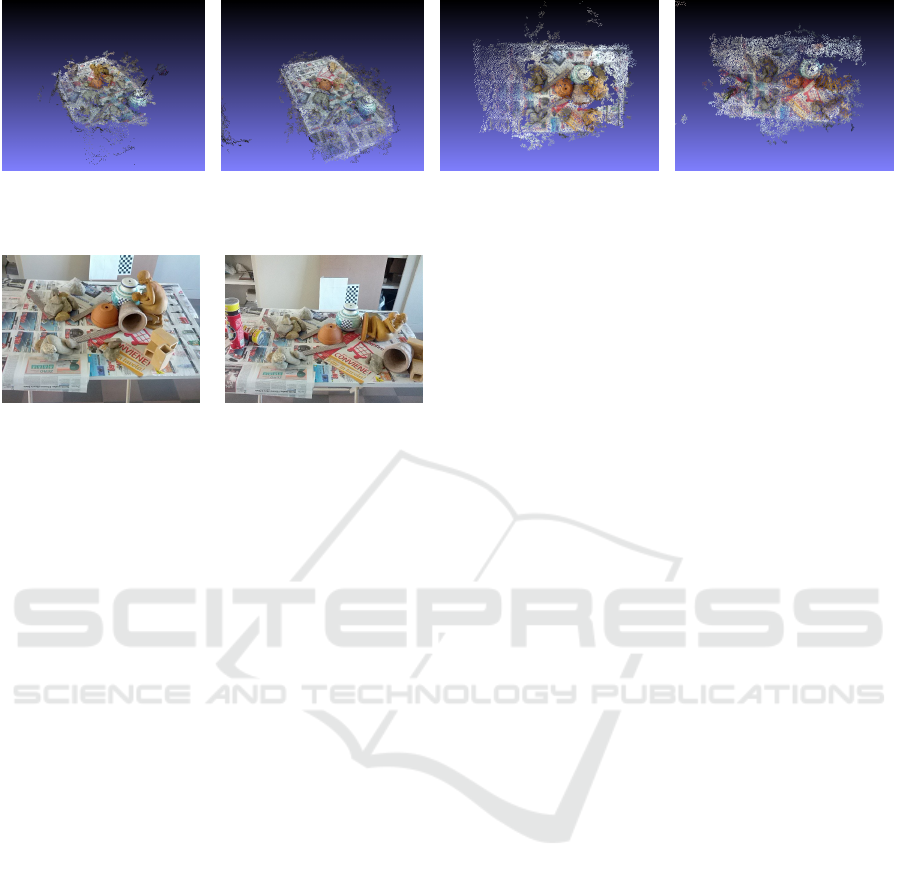
(a) (b) (c) (d)

Figure 5: Dense 3D reconstructions obtained respectively from (a) I

, (b) I

, (c) I

, and (d) I

(a) (b)

Figure 4: Frames from the sequences I

(a) and I

(b). Two

cylindrical cans were added in the left side, the statue on the

right was laid down, and the jar, the rocks, and the bricks

were moved to a different position.

All images were acquired with a consumer camera

with resolution 640x480; for I

and I

, 22 and 30 ima-

ges were recorded respectively, while I

and I

are

made of 22 and 18 images. Parameters were selected

experimentally as follows: α is equal to the average

number of points per voxel computed over D

and D

β = 0.5, γ = 10, and µ = 75.

3.1 Qualitative Results

Figure 5 shows the dense 3D models obtained with

SfM for the four image collections described before.

To visually appreciate the detected changes, in Fig. 6

we present the obtained 3D heat-maps for the ﬁrst (I

vs I

) and the second (I

vs I

) test setups. Hotter areas

indicate a higher probability of occurred change.

As clear from the inspection of Fig. 6a, the remo-

ved jar and statue correspond to the hottest areas of

the heat-map for the ”Object removal” test. Similarly,

all the relevant objects of the ”Object insertion and

displacement” test are correctly outlined by red areas

in Fig. 6b. However, some false positives are present

in both the 3D heat-maps: This is probably due to

errors in the 3D reconstruction. Indeed, these false

positives appear mostly on peripheral areas of the re-

construction, related to background elements that are

under-represented in the image collection (the acqui-

sition was made circumnavigating the area of interest)

and thus reconstructed in 3D with less accuracy.

In order to better assess the performance of the

proposed method, and also to observe the impact of

the false positives visible in the heat-maps, we com-

plemented the above qualitative analysis with a quan-

titative one.

3.2 Quantitative Results

Ground-truth (GT) masks highlighting the changes

occurred between the two image sequences were ma-

nually constructed. Fig. 7 reports two example of GT

masks: Fig. 7b shows the changes between I

and I

reported in the reference system of I

, while Fig. 7d

depicts the comparison of I

and I

, in the coordinate

frame of I

The GT masks were used to evaluate the Receiver

Operating Characteristic (ROC) curve and assess the

performance of our method for both the tests at hand.

Fig. 8 shows the performance obtained with the

sparse 2D change maps. In Figure 9 ROC curves

obtained for I

vs I

and I

vs I

are reported. The

values of the Area Under the ROC Curve (AUC) are

respectively 0.76 and 0.89.

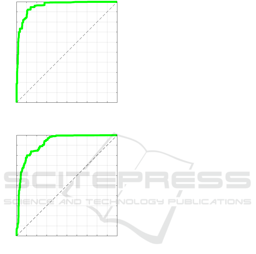
Improving the 2D change maps as described

in Sect. 2.3 by exploiting superpixel segmentation

(see Figs. 10a and 10c), yields denser and smoother

maps—see Figs. 10b and 10d. The corresponding

ROC curves are shown in Figs. 11a and 11b respecti-

vely. AUC values are 0.96 for I

vs I

, and 0.92 for I

vs I

. With the improved change maps, the AUC for

the ”Object insertion and displacement” test increases

only by 3%, while in the ”Object removal” test the

AUC increases by almost 20% (0.19). This is due to

the fact that the reconstructed 3D maps from I

and

are denser that those obtained from I

and I

(see

again Fig. 5). As a result, the sparse 2D change map

for the ”Object insertion and displacement” test is of

better quality than its homologous for the ”Object

removal” test. For completeness, we report in Table 1

True Positive (TP), False Positive (FP), True Negative

(TN), and False Negative (FN) values obtained at

the ROC cut-off point that maximizes the Younden’s

VISAPP 2019 - 14th International Conference on Computer Vision Theory and Applications

764

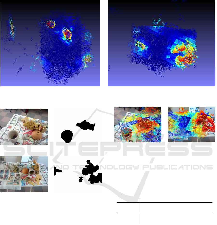
(a) (b)

Figure 6: Heat-maps obtained from (a) I

vs I

and (b) I

vs I

(a) (b)

Figure 7: Example of ground-truth masks: (a) an image

from I

and (b) its GT mask, (c) an image from I

and (d)

its GT mask. It is worth noting that, while the GT mask

of I

vs I

is simply obtained by highlighting the removed

object only, in the mask for I

vs I

highlighted areas have to

account for removed, displaced or inserted objects. For this

reason, the GT map (d) was obtained by fusing the masks of

with those of I

—after having performed view alignment

based on the registered 3D models.

Index, i.e.

max{Sensitivity + Speci ficity − 1} =

max{T PR − FPR}

(1)

where TPR and FPR are the True Positive Rate and

the False Positive Rate, respectively.

(a) (b)

Figure 8: Sparse 2D change maps obtained by projecting

the computed 3D heat-map onto a reference frame of I

(a),

and I

(b).

Table 1: True Positive (TP), False Positive (FP), True Nega-

tive (TN), and False Negative (FN) percentage obtained at

the ROC cut-off point for each test sequence, plus the rela-

ted AUCs. The subscript

SPX

indicates the improved change

maps using superpixel segmentation.

Scene TP FP TN FN AUC

vsI

0.12 0.04 0.74 0.10 0.76

vsI

SPX

0.13 0.10 0.76 0.01 0.96

vsI

0.23 0.11 0.61 0.05 0.89

vsI

SPX

0.15 0.10 0.72 0.03 0.92

4 CONCLUSIONS AND FUTURE

WORK

In this paper, a vision-based change detection met-

hod based on three-dimensional scene comparison

was presented. Using as input two 3D reconstructions

of the same scene obtained from images acquired at

different times, the method estimates a 3D heat-map

that outlines the occurred changes. Detected chan-

ges are also highlighted into the image space using a

2D change map obtained from the 3D heat-map. The

Structural Change Detection by Direct 3D Model Comparison

765

0 0.1 0.2 0.3 0.4 0.5 0.6 0.7 0.8 0.9 1

FPR

0.1

0.2

0.3

0.4

0.5

0.6

0.7

0.8

0.9

TPR

(a)

0 0.1 0.2 0.3 0.4 0.5 0.6 0.7 0.8 0.9 1

FPR

0.1

0.2

0.3

0.4

0.5

0.6

0.7

0.8

0.9

TPR

(b)

Figure 9: ROC curves obtained from the sparse 2D change

map. In (a) ROC for I

vs I

achieving an AUC of 0.76. In

(b) ROC for I

vs I

achieving an AUC of 0.89.

method works in two steps. First, a rigid transfor-

mation to align the 3D reconstructions is estimated.

Then, change detection is evaluated by comparing lo-

cally corresponding areas. Three criteria are used to

assess the occurrence of a change: a quantity crite-

rion based on the number of 3D points, an orientation

criterion that exploits the normal vector orientations

to assess shape similarity, and an occupancy criterion

to evaluate the local spatial distribution of 3D points.

As a by-product, a 4D map (space plus time) of the

environment can be constructed by overlapping the

(a) (b)

Figure 10: Superpixel segmentation examples and impro-

ved 2D change maps.

aligned 3D maps. Qualitative and quantitative results

obtained from tests on two complex datasets show the

effectiveness of the method, that achieves AUC values

higher than 0.90.

Future work will address a further improvement

of the 2D change map, based on the introduction of

surface (3D mesh) information into the computational

pipeline.

REFERENCES

Achanta, R., Shaji, A., Smith, K., Lucchi, A., Fua, P., and

Ssstrunk, S. (2012). Slic superpixels compared to

state-of-the-art superpixel methods. IEEE Transacti-

ons on Pattern Analysis and Machine Intelligence,

34(11):2274–2282.

Alcantarilla, P. F., Stent, S., Ros, G., Arroyo, R., and Gher-

ardi, R. (2016). Street-view change detection with de-

convolutional networks. In Proceedings of Robotics:

Science and Systems, AnnArbor, Michigan.

Besl, P. J. and McKay, N. D. (1992). A method for regis-

tration of 3-d shapes. IEEE Transactions on Pattern

Analysis and Machine Intelligence, 14(2):239–256.

Brown, L. G. (1992). A survey of image registration techni-

ques. ACM Comput. Surv., 24(4):325–376.

Cavallaro, A. and Ebrahimi, T. (2001). Video object ex-

traction based on adaptive background and statistical

change detection. In Proc.SPIE Visual Communicati-

ons and Image Processing, pages 465–475.

Collins, R. T., Lipton, A. J., and Kanade, T. (2000). Intro-

duction to the special section on video surveillance.

IEEE Transactions on Pattern Analysis and Machine

Intelligence, 22(8):745–746.

Dai, X. and Khorram, S. (1998). The effects of image misre-

gistration on the accuracy of remotely sensed change

VISAPP 2019 - 14th International Conference on Computer Vision Theory and Applications

766

0 0.1 0.2 0.3 0.4 0.5 0.6 0.7 0.8 0.9 1

FPR

0.1

0.2

0.3

0.4

0.5

0.6

0.7

0.8

0.9

TPR

(a)

0 0.1 0.2 0.3 0.4 0.5 0.6 0.7 0.8 0.9 1

FPR

0.1

0.2

0.3

0.4

0.5

0.6

0.7

0.8

0.9

TPR

(b)

Figure 11: ROC curves obtained from the improved 2D

change maps. In (a) ROC for I

vs I

achieving an AUC

of 0.96. In (b) ROC for I

vs I

achieving an AUC of 0.92.

detection. IEEE Transactions on Geoscience and Re-

mote Sensing, 36(5):1566–1577.

Fanfani, M., Bellavia, F., and Colombo, C. (2016). Accurate

keyframe selection and keypoint tracking for robust

visual odometry. Machine Vision and Applications,

27(6):833–844.

Fanfani, M., Bellavia, F., Pazzaglia, F., and Colombo, C.

(2013). Samslam: Simulated annealing monocular

slam. In International Conference on Computer Ana-

lysis of Images and Patterns, pages 515–522. Sprin-

ger.

Furukawa, Y. and Ponce, J. (2010). Accurate, dense, and ro-

bust multiview stereopsis. IEEE Transactions on Pat-

tern Analysis and Machine Intelligence, 32(8):1362–

1376.

Horn, B. K. P. (1987). Closed-form solution of absolute

orientation using unit quaternions. Journal of the Op-

tical Society of America A, 4(4):629–642.

Mani, G. F., Feniosky, P. M., and Savarese, S. (2009). D

– A 4-dimensional augmented reality model for au-

tomating construction progress monitoring data col-

lection, processing and communication. Electronic

Journal of Information Technology in Construction,

14:129 – 153.

Palazzolo, E. and Stachniss, C. (2017). Change detection

in 3D models based on camera images. In 9th Works-

hop on Planning, Perception and Navigation for In-

telligent Vehicles at the IEEE/RSJ Int. Conf. on Intel-

ligent Robots and Systems (IROS).

Pollard, T. and Mundy, J. L. (2007). Change detection in

a 3-d world. In 2007 IEEE Conference on Computer

Vision and Pattern Recognition, pages 1–6.

Qin, R. and Gruen, A. (2014). 3D change detection at street

level using mobile laser scanning point clouds and ter-

restrial images. ISPRS Journal of Photogrammetry

and Remote Sensing, 90:23 – 35.

Radke, R. J., Andra, S., Al-Kofahi, O., and Roysam, B.

(2005). Image change detection algorithms: a sys-

tematic survey. IEEE Transactions on Image Proces-

sing, 14(3):294–307.

Sakurada, K., Okatani, T., and Deguchi, K. (2013). De-

tecting changes in 3D structure of a scene from multi-

view images captured by a vehicle-mounted camera.

In Computer Vision and Pattern Recognition (CVPR),

2013 IEEE Conference on, pages 137–144. IEEE.

Sch

onberger, J. L. and Frahm, J.-M. (2016). Structure-

from-motion revisited. In Conference on Com-

puter Vision and Pattern Recognition (CVPR).

https://colmap.github.io/.

Szeliski, R. (2010). Computer Vision: Algorithms and

Applications. Springer-Verlag New York, Inc., New

York, NY, USA, 1st edition.

Taneja, A., Ballan, L., and Pollefeys, M. (2011). Image

based detection of geometric changes in urban envi-

ronments. In 2011 International Conference on Com-

puter Vision, pages 2336–2343.

Taneja, A., Ballan, L., and Pollefeys, M. (2013). City-scale

change detection in cadastral 3D models using ima-

ges. In 2013 IEEE Conference on Computer Vision

and Pattern Recognition, pages 113–120.

Toth, D., Aach, T., and Metzler, V. (2000). Illumination-

invariant change detection. In 4th IEEE Southwest

Symposium on Image Analysis and Interpretation, pa-

ges 3–7.

Toyama, K., Krumm, J., Brumitt, B., and Meyers, B.

(1999). Wallﬂower: principles and practice of back-

ground maintenance. In Proceedings of the Seventh

IEEE International Conference on Computer Vision,

volume 1, pages 255–261 vol.1.

Wu, C. (2013). Towards linear-time incremental struc-

ture from motion. In 2013 International Confe-

rence on 3D Vision - 3DV 2013, pages 127–134.

http://ccwu.me/vsfm/.

Structural Change Detection by Direct 3D Model Comparison

767