Elimination of Boundary Effects at the Numerical Implementation of
Continuous Wavelet Transform to Nonstationary Biomedical Signals
S. V. Bozhokin, I. B. Suslova and D. A. Tarakanov
Peter the Great Saint-Petersburg Polytechnic University, Polytechnicheskaya 29, Saint-Petersburg, Russia
Keywords: Continuous Wavelet Transform, Boundary Effects, Nonstationary Heart Tachogram.
Abstract: The main objective of the paper is to develop an algorithm improving the situation with boundary effects at
the numerical implementation of continuous wavelet transform, what makes it possible to hold down
important information in the study of many nonstationary biological signals. As a basis for the research, we
propose the mathematical model of nonstationary signal (NS) with a complex amplitude variation in time.
Such signals show peaks near the beginning and end of the observation period. The model leads to the
analytical expression for continuous wavelet transform (CWT). Thus, we get to know how boundary effects
relate to the finiteness in time of the mother wavelet function. To avoid boundary effects arising at the
procedure of numerical wavelet transform, we develop the algorithm of signal time shift (STS). The results of
analytical solution and numerical CWT calculation with and without the use of STS show the benefit of using
STS in the processing of nonstationary signals. We have applied the technique to the study of nonstationary
heart tachogram and discovered heart activity bursts in different spectral ranges, which appear and disappear
at different time moments.
1 INTRODUCTION
The technique of CWT (continuous wavelet
transform) allows us to develop a system of
quantitative parameters for analysing nonstationary
(NS) signals, with statistical and spectral properties
changing in time (Mallat, 2008), (Cohen, 2003),
(Advances in Wavelet, 2012), (Chui and Jiang, 2013),
(Addison, 2017), (Hramov, 2015). The first important
operation in the wavelet theory is the scaling
procedure, in which we change the region of wavelet
function localization in frequency. The second step is
the shift operation, in which we change the
localization of wavelet function in time. In this way,
we can clearly reveal the amplitude-frequency
properties of the signals under study. CWT represents
three-dimensional surface
 
,Vt
depending on
frequency

and time
t
. Analytical CWT
calculations using the Morlet mother wavelet
function show that for harmonic signal
0
Z( ) cos(2 )t f t
(
0
f
is the frequency), the
maximum of
 
,Vt
is reached at
0
f
, and this
maximal value does not depend on
t
. In the case of
two infinite harmonic signals with frequencies
1
f
,
2
f
and the same amplitude, we observe the peaks of
ridges with the same amplitude
 
,Vt
at points
1
f
and
2
f
(Bozhokin, 2012), (Andreev et al.,
2014), (Bozhokin and Suslova, 2013), (Bozhokin and
Suslova, 2015), (Bozhokin et al., 2017). The majority
of CWT studies use numerical calculations. In this
case, the question arises of how accurately CWT
reproduces the properties of
()Zt
given in the finite
interval
[0, ]tT
(
T
is the time of observation). The
shortcoming of CWT is the finite temporal resolution
of the mother wavelet function. This causes boundary
effects near the initial and final moments of time,
where we can observe significant differences in the
amplitude-frequency properties of the original signal
()Zt
and its CWT image
 
,Vt
. To correct this
drawback and improve the resolution of low
frequency signal components in the case of short
signal duration, the authors of (Tankanag and
Chemeris, 2009), (Podtaev et.al.,2008), (Boltezar and
Slavic, 2004), (Ulker-Kaustell and Karoumi, 2011)
undertook a modification of CWT algorithm. The
work (Cazelles et al.,2008) presents the discussion of
boundary effects depending on the type of the mother
wavelet function. The numerical estimation of
Bozhokin, S., Suslova, I. and Tarakanov, D.
Elimination of Boundary Effects at the Numerical Implementation of Continuous Wavelet Transform to Nonstationary Biomedical Signals.
DOI: 10.5220/0007254900210032
In Proceedings of the 12th International Joint Conference on Biomedical Engineering Systems and Technologies (BIOSTEC 2019), pages 21-32
ISBN: 978-989-758-353-7
Copyright
c
 2019 by SCITEPRESS – Science and Technology Publications, Lda. All rights reserved
21

boundary effects at CWT for real experimental
nonstationary signals was carried out in (Tankanag
and Chemeris, 2009), (Podtaev et.al.,2008), (Boltezar
and Slavic, 2004), (Ulker-Kaustell and Karoumi,
2011).
When analysing non-stationary signals in
medicine, the development of quantitative parameters
to describe heart rate variability is of great
importance. Heart rate variability (HRV) inferred
from the analysis of a tachogram—a series of RR
intervals between heart contractions—is known as an
important index in cardio-vascular system
assessment (CVS) (Addison, 2017), (Baevskii et al,
2002), (Anderson et al, 2018), (Bhavsar et al. 2018),
(Hammad et al, 2018). However, the statistical
parameters of HRV (RRNN, SDNN, RMSSD), the
spectral characteristics of cardio intervals employing
the Fourier transform (ULF, VLF, LF, HF), and the
histogram methods given in the Standards can be used
only in stationary situations. The condition of
stationarity, meaning the repetition of statistical and
spectral characteristics of the cardio signal taken
arbitrarily over any time segment, is not fulfilled in
the majority of cardiac situations. In particular, it is
true for the passive tilt test used for complex
assessment of the cardiovascular system (CVS) to
elucidate the mechanisms of its autonomous
regulation. This test allows good standardization. The
passive tilt test is performed on a special automated
tilt table, which brings the body from the horizontal
into the vertical position. There are two types of
orthostatic tests, in which the human head rises (HUT
–head up table) and in which the human head falls
(HDT –head down table). Tilt tests are used to
determine the tolerance of the organism to abrupt
changes of body position in occupational selection
(pilots and cosmonauts), prescription of drugs that
affect blood redistribution in diagnosing neuro-
circulatory disorders, and elucidation of the
mechanisms of functional impairment of the
autonomous system (ANS), in particular, detecting
patients with neuro -cardiac fainting spells (syncope).
The wavelet theory has been successfully applied
in HRV studies (Addison, 2017), (Keissar at al.
2009), (Ducla-Soares et al, 2007). Most HRV studies
based on the wavelet theory use the models of
amplitude-modulated signals, i.e., when the regular
sampling interval ∆t coincides with the mean RR
interval (∆t = RRNN). However, in many actual
situations, where it is necessary to analyze accurately
the cardiac arrhythmia, the time points of heartbeats
are spaced very irregularly. Thus, developing of new
models to study the transitional processes in the heart
rhythm, which occur very often, for example, at tilt
tests, remains a pressing problem.
In the present paper, we develop an algorithm to
eliminate boundary effects in the numerical
implementation of the continuous wavelet transform.
To solve this problem, we introduce the mathematical
model of a signal with complextime variation in the
amplitude
 
At
. The model specifies the time
behaviour of the amplitude, as well as the occurrence
of peaks near the beginning and end of the
observation period. This model allows us to obtain the
analytical solution for the wavelet transform
 
,Vt
and compare it with the given signal amplitude
 
At
. To eliminate boundary effects arising at the
numerical procedure of CWT, we propose the
algorithm of signal time shift (STS).
The aim of the work is to use the developed
method STS together with the technique of CWT for
the quantitative description of non-stationary heart
rate variability. In the model we propose here, the
HRV signal is a superposition of the Gaussian peaks
of the same amplitude. The centers of heart beats
separated by
n
RR
time intervals are located on a
substantially irregular grid, which is characterized by
time points
n
t
, where
1n n n
t t RR


, n = 1, 2, 3,
…, N – 1, and
00
t RR
. These time points strictly
correspond to the time points of the actual RR
intervals. Our tachogram model considers frequency
modulated signals and provides an analytical solution
using CWT with the Morlet mother wavelet function.
The maximal CWT value corresponds the value of
local frequency function
 
max
Ft
Applying the
second CWT (DCWT) for the signal
 
max
Ft
allows
us to study both aperiodic and oscillory movements
of the local frequency in ULF,VLF, LF, as well as the
HF spectral ranges (Bozhokin and Suslova, 2013),
(Bozhokin and Suslova, 2014), (Bozhokin et al,
2018).
2 METHODS
2.1 Mathematical Model of
Nonstationary Signal
We consider nonstationary signal
()Zt
with the
amplitude varying strongly in time. The characteristic
feature of the proposed model is the complex
behavior of the signal amplitude at time interval
boundaries. We represent
()Zt
as a superposition of
BIOSIGNALS 2019 - 12th International Conference on Bio-inspired Systems and Signal Processing
22

N elementary nonstationary signals (ENS) centered in
the points
L
tt
and determined by the system of L
parameters:
 
1
0
( ) .
N
LL
L
Z t z t t




(1)
ENS signal
 
LL
z t t
in (1) has the shape of the
Gaussian envelope of oscillating function (Bozhokin,
2012)
 
 
 
2
2
exp cos 2 .
2
4
L
L
L L L L L
L
L
tt
b
z t t f t t



      






(2)
Five parameters
( ; ; ; ; ),
L L L L L
L b f t  
(3)
which determine the ENS, are: the amplitude
L
b
having the dimensions
()volt second
; the frequency
of oscillations
L
f
in (Нz); the characteristic size
L

of
signal time localization in (s); the initial phase
L

in
radians. Hereinafter, we assume that the condition
1
LL
f  
holds for all ENS considered in the present
paper. This means that time interval
L

, which equals
the characteristic scale of amplitude decreasing, covers
many oscillation periods
1/
LL
Tf
.
As an example, we consider the signal
()Zt
(1)
represented by four ENS (2) at
L
=0,1,2,3. Suppose
the frequencies of all signals equal
2
L
f 
Hz, and their
phases have zero values.
Table 1 displays all other parameters of the ENS.
The parameters in Table 1 are chosen in such a way
that the total signal has the form
 
0
( ) ( )cos 2 ,Z t B t f t
(4)
where
0
f
=2Hz.
Table 1.
The parameters of four ENS in (1)
(s)
(s)
(s)
0
–0.3
3
0.75
1
25
5
2
25
4.5
3
–0.3
47
0.75
The value of
()Bt
can be represented in the form
 
 
2
1
2
0
1
exp
2
4
N
L
L
L
L
L
tt
b
Bt












.
(5)
Let us introduce the notations
( ) ( )A t B t
,
( )/
m
A t A
,
(6)
where
m
A
is the maximal value of the amplitude.
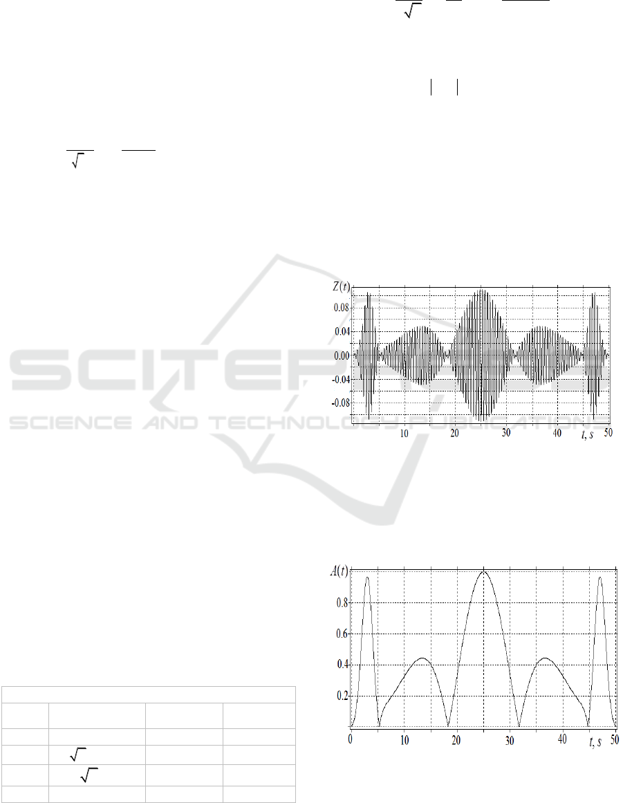
Fig.1 shows the proposed model (1) of the signal. It
is essential that the signal has the points of zero
amplitude. Besides, the graph shows two high peaks
with narrow localization
0

=0.75 s and
3

= 0.75 s at
the beginning
3t 
s, and at the end
47t 
s of the
process.
Fig.2 shows the behavior of
( )/
m
A t A
within the
interval
0 ( )/ 1
m
A t A
.
Figure 1: Time dependence of the signal
()Zt
(1) with the
parameters given in Table 1.
It is important to emphasize that the proposed model
allows us to set the amplitude exactly. Hereupon, the
model gives the analytical solution for CWT.
Figure 2: Dependence of
( )/
m
A t A
in time.
L
L
b
L
t
L

10 
10
Elimination of Boundary Effects at the Numerical Implementation of Continuous Wavelet Transform to Nonstationary Biomedical Signals
23

Further study will focus on computing CWT,
formulating the criteria for determining how correctly
CWT shows the time behavior of the amplitude
()At
,
and eliminating boundary effects in CWT
implementation.
2.2 Continuous Wavelet Transform
The continuous wavelet transform
 
,Vt
(CWT)
maps nonstationary signal
 
Zt
with varying time-
frequency structure on time-frequency plane
(Addison, 2017), (Wavelet in Physics, 2004):
     
 
*
,,V t Z t t t dt


  
     

(7)
where
 
x
is the mother wavelet function, and
symbol * means complex conjugation. The mother
wavelet
 
x
should be localized near the point
0x 
, have the unit norm value, and zero mean value
calculated over the interval
x   
. The adaptive
Morlet mother wavelet function (AWM), which we
introduced in (Bozhokin et al. 2017), satisfies all
these properties. The formulas for AMW and its
Fourier image are
   
 
2
2
2
exp exp 2 exp ,
2
mm
x
x D ix
m


     





(8)
 


2
22
( ) exp 1 1 exp 2 ,
mm
mm
D
F F F



      




(9)
 
 
1/4
2
2
2
.
3
1 2exp exp 2
2
m
m
mm
D






     





(10)
The value
m
in (8)-(10) plays the role of a control
parameter, while
2
m
m  
. The parameter of
localization
x

, which indicates the extension of
 
x
along x-axis, and
F

, which corresponds to
the extension of Fourier spectrum
 
F
(Mallat,
2018), (Chui and Jiang, 2013) along the frequency
axis, have the values
/2
x
m
, and
1/ ( 8 ).
F
m  
Their product is close to the lowest
value
1/ (4 ).
xF
   
The values of
x

and
F

vary with the change in
.m
Thus, we get the
opportunity to vary the time and spectral resolution of
the signals under study. At
1m 
we obtain the
formula for the ordinary Morlet mother wavelet
function. If the characteristic length of
 
x
is
/2
x
m
, the characteristic time moments, which
make the main contribution to the integral (7), satisfy
the relation
.
xx
t t t


   

(11)
Thus, AMW (8) behaves like a varying window
depending on the control parameter. The window
width automatically becomes large for small
frequencies and small for the large ones.
We note, that the wavelet transform (7) with the
mother wavelet (8) for elementary nonstationary
signals (2), with the amplitude varying in time and
constant frequency, can be calculated analytically
(Bozhokin et al, 2017). In this case, the maximum of
 
,
L
Vt
in frequency is achieved at the point, and the
time behavior of
 
,
L
Vt
reproduces that of the
signal amplitude. We can easily find the analytical
expression of CWT for the superposition (1). The
characteristic lengths
(CWT)
t

and
(CWT)


of
 
2
,
L
Vt
along the time and frequency axes have
the values:
(CWT)
2 2 2
1 / (2 ),
t L L L
mf    
(12)
(CWT) 2 2 2
1 2 / / (4 ).
L L L
fm

    
(13)
It is easy to derive two limiting cases of these
formulas (
LL
mf 
and
LL
mf 
).
2.3 Wavelet Analysis of Mathematical
Model of Nonstationary Signal
After applying CWT with
1m 
to (1), we can
observe that at
L
f
the time behavior
   
 
2
2
2
, exp / 2
L L L L
V f t t t

   


exactly reproduces
the time behavior of
 
2
At
. If the control parameter
LL
mf 
, then the behavior of
 
2
,
LL
V t t
exactly repeats the behavior of power spectrum
   
2
L
Pz  
, and
()CWT


exactly coincides
with
(0)


, which characterizes the width of ENS (2)
power spectrum, i.e.
(CWT) (0)
1/ (4 )
L
    
.
Fig.3 shows the complex amplitude and frequency
properties of the signal.
BIOSIGNALS 2019 - 12th International Conference on Bio-inspired Systems and Signal Processing
24

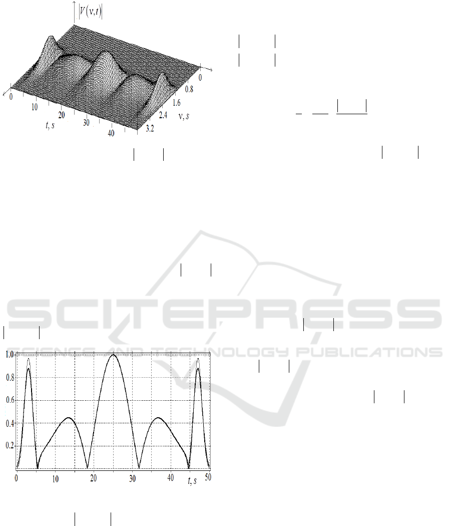
Figure 3: Analytical dependence of
 
,Vt
on frequency
()Hz
and time
()ts
for the signal
()Zt
.
At
L
t
=3s (
L
=0) and
L
t
=47s (
L
=3) corresponding
to the sharp peaks, we have wide frequency
distribution. It is due to the fact that the length
L

=0.75s of these peaks (
L
=0,
L
=3) is much smaller
than the lengths of two other peaks
L

=5s (
L
=1) and
L

=4.5s (
L
=2). To find out how
 
,Vt
reproduces the behavior of the signal amplitude
 
,At
we make a cross-section of the surface at
0
f
along the time axis. Fig.4 shows the cross-section of
 
0
,V f t
in comparison with
 
At
.
Figure 4: Comparison of time behavior for
 
At
(thin line)
and cross section of
 
0
,V f t
(bold line) at
1m 
.
In Fig. 4 we can see that the curves diverge only in a
close neighborhood of peaks
L
t
=3s (
L
=0) and
L
t
=47s (
L
=3). It is because these two peaks are located
at the beginning and at the end of the interval
[0, ]T
,
where the condition
1
LL
f  
is violated (
0
f
=2Hz;
0

=
3

=0.75s). The curves nearly coincide at all
other points of the interval
[0, ]T
, where
T
=50s. We
conclude that for
1
LL
f  
, the curves
 
At
and
 
0
,V f t
are similar. To characterize the deviation of
 
0
,V f t
from
 
At
, we introduce the parameter of
mean square deviation by the formula
 
 
2
0
2
0
;
1
,
T
t
mm
V f t
At
dt
T A V

  




(14)
where
m
V
is the maximal value of
 
0
,V f t
within
the interval
[0, ]T
. Thus, CWT with
1m 
is well
suited to describe the time variation of amplitude
 
At
for some specific moments, in which
 
At
=0
(Fig.2).
3 RESULTS
3.1 Boundary Effects in the Analysis of
Spectral Properties
The foregoing results are based on the analytical
expressions for
 
,Vt
and
 
At
for the proposed
mathematical model of nonstationary signal. For real
signals, we are to carry out numerical calculations to
find
 
,Vt
. In this case, we face the problem of
boundary effects. Let us determine the influence of
boundary effects in calculating
 
,Vt
(Bozhokin
and Suslova, 2013). Boundary effects can appear at
both the left
(0 )
off
tt
and the right
()
off
T t t T  
ends of the observation interval
T
. The value of
off
t
will be determined later. The
reason is the finite value of wavelet’s length
x

,
which leads to significant errors in numerical CWT
calculation. To eliminate the errors, we take the
values of
 
,Vt
in these intervals equal to zero.
Naturally, we lose the valuable information on the
time-frequency behavior of the signal within these
intervals. How can you keep this information?
Let us formulate the problem of finding the
minimal value
min

of frequency that will allow us
to determine CWT correctly. Analyzing (11), we
conclude that in the initial interval
[0, ]
off
t
, the
Elimination of Boundary Effects at the Numerical Implementation of Continuous Wavelet Transform to Nonstationary Biomedical Signals
25

min
2
.
x
off
t



(15)
A similar formula can be obtained near the right-
hand boundary
;
off
T t T



of the signal. To
determine
min

correctly, we need
n
(
1n 
)
periods of frequency oscillations with the duration of
min
1/
that can be placed within the remaining time
interval [
2
off
Tt
]. The observation interval T
consists of two boundary sections with the lengths
min
4/
x

and
min
/n 
(the interval to determine
CWT correctly). Then we have
min
4
.
x
n
T


(16)
Taking into account the boundary effects leads to the
value of
min

approximately
4
x
n
times
largerthan
min
1/fT
used in the Fourier analysis.
After determining
min

(16), we can calculate the
value of
off
t
(15).
To eliminate boundary effects, we propose an
algorithm, which we call Signal Time Shift (STS).
Knowing the value
min

(16), we can extend the
interval of signal observation from
T
to
1
T
. The
beginning of the interval
T
(
0t 
) is transferred
into the point
min
t
, and the initial interval
 
min
0;t
,
which enters a new time period
1
T
, should be filled
with the initial constant values of the signal
 
0.Zt
We are to choose the value of
min
t
larger
than the initial section, where we can observe the
boundary effects, i.e.
min min
2.5 /
x
t   
. This value
is larger than
off
t
(
min
1.25
off
tt
). We also fill the
new finite interval
 
1 min 1
;T t T
with the constant
values
 
Z t T
of the signal. The central interval
min 1 min
[ ; ]t T t
at
1
TT
has the duration
.T
It
exactly repeats all the values of the investigated
signal. Thus, the values of
 
Zt
are located in the
central part of the new interval
1
T
outside the
boundary effect zone.
The primary interval
T
is shown in the upper part of
Fig.5. This interval consists of two boundary sections
(in black) with the duration
min
2 4 /
off x
t   
plus
the section with the duration
min
/n 
. The lower
Figure 5: The upper drawing corresponds to the interval
T
with two boundary sections marked in black; the lower
drawing corresponds to
1
T
.
drawing in Fig.5 shows the enlarged interval
1
T
,
which consists of the central section
T
with all values
of
 
Zt
(in grey) and two sections of total duration
min min
2 5 /
x
t   
with the boundary values of
 
Zt
. We make equal the minimum frequency values
   
min min 1
TT  
for
T
and
1 min
5/
x
TT   
. In this case, the number of periods
 
nT
and
 
11
nT
for correct determination of the frequency
min

are
related to each other as
   
11
5
x
n T n T  
. The
next step in STS algorithm is numerical calculations
of CWT in the interval
1
[0, ]T
. Then, we eliminate all
the values of
 
,Vt
located at the beginning of
 
min
0;t
and at the end of
min 1 min
[ ; ]t T t
. The
subsequent shift of start timing from point
min
tt
to
the point
t
=0 restores the initial observation interval
 
0;tT
, and allows us to compare the values of
 
,Vt
with the true behavior of the signal
 
Zt
taking into account the boundary effects.
Let us compare the analytical behavior of
 
At
(Fig.2) with that of
 
0
,V f t
(CWT) (Fig.4),
numerical implementation
 
(num)
0
,V f t
of CWT
without the procedure of signal time shift (STS), and
the numerical implementation
 
()
0
,
sts
V f t
of CWT
with the use of STS. All calculations are carried out
for the model (1)-(2) and the parameters given in
Table 1. Numerical calculations are made for the
Morlet wavelet with
1m 
, the characteristic length
x

=1, the number of oscillation periods
10n 
. In
BIOSIGNALS 2019 - 12th International Conference on Bio-inspired Systems and Signal Processing
26

this case,
T
=50s,
min

=0.28Hz,
off
t
=7.14s,
min
t
=8.93s,
1
T
=61.76s.
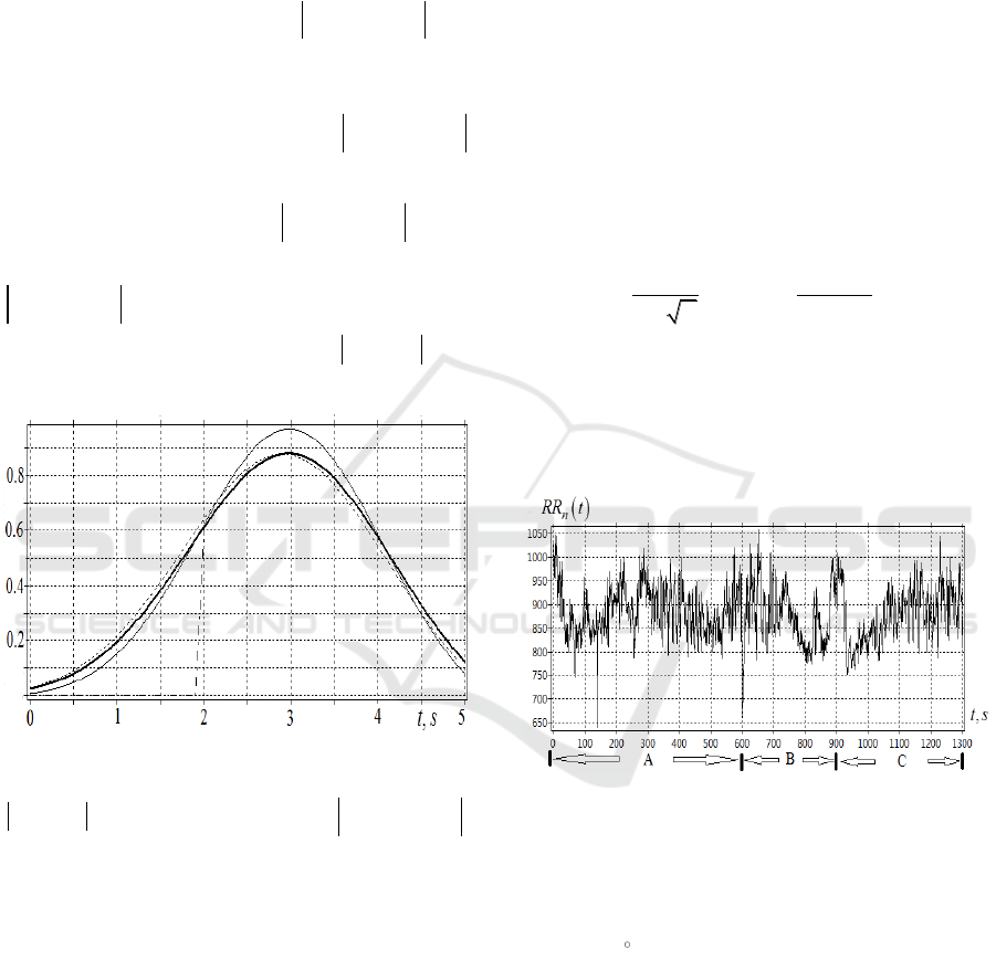
Fig.6 represents a small fragment of the signal near
the beginning to demonstrate the boundary effects.
The duration is 5s. In Fig.6 the dash-dot line shows
CWT calculated numerically
 
(num)
0
,V f t
, in
which the boundary effects appear. For the
frequencies

1 Hz, the cut-off time is
off
t 
2s. We
observe strong differences between
 
(num)
0
,V f t
and
 
At
at times
0
off
tt
. This requires us to take
as zeros the wrong values of
 
(num)
0
,V f t
in the
interval
02ts
. The dot line represents the result
 
()
0
,
sts
V f t
of applying STS method. This line
reproduces the analytical behavior of
 
0
,V f t
quite
well.
Figure 6: Thin line ‒
 
At
; bold line – analytical
 
0
,V f t
; dash-dot line – numerical
 
(num)
0
,V f t
,
which takes zero values at small times; dot line – numerical
with the use of signal time shift.
Thus, the numerical implementation together with
STS method allows us to save the important
information about the amplitude–frequency behavior
of the signal near the beginning and the end of the
observation interval. The signal time shift allows us
to consider all the time points of the signal under
study.
3.2 STS Algorithm in the Analysis of
Heart Tachоgram
The method of eliminating boundary effects (STS),
developed in the previous section, can be applied in
the study of non-stationary signal representing the
heart tachogram.
In contrast to the traditional approach of simulating
the tachogram as an amplitude modulated signal with
the points equidistant in time, we consider it as a
frequency-modulated signal (Bozhokin and Suslova,
2013). We represent the heart tachogram signal as a
set of identical Gaussian peaks, whose centers
n
t
are
located on an uneven grid of times, and coincide in
time with the true moments of heart beats:
1n n n
t t RR


, n = 1, 2, 3, …, N – 1, and
00
t RR
.
The width
0
20  
ms of each Gaussian peak is equal
to the width of the QRS complex.
 
 
2
1
2
0
0
0
1
exp
2
4
N
n
n
tt
Zt











.
(17)
Such a model makes it possible to obtain the
analytic expression for
 
,Vt
(7). Fig.7 shows
human heart tachogram registered during Head Down
Tilt Test. It consists of three stages: A,B,C.
Figure 7: Dependence of heart bear interval
n
RR
on time
()t ms
.
Stages A,C correspond to the horizontal position of
the table. Stage B is the lowering of the table with a
turn of
30
, which leads to the transients in the
frequency of heart beats.
Let us consider the experimental tachogram
(Fig.7) registered during head-down tilt test (HDT)
The duration of intervals
n
RR
between the centers of
heartbeats changes. Stage B, when the HDT takes
place, lasts 300 s (
600 900t
s). For the proposed
model of tachogram (17), the Gaussian peaks (17) are
centered at the times
n
t
when heartbeats occur:
1n n n
t t RR


, n = 1, 2, 3, .. N –1, and
00
t RR
.
Elimination of Boundary Effects at the Numerical Implementation of Continuous Wavelet Transform to Nonstationary Biomedical Signals
27

Substituting these
n
t
into (17), we obtain the
frequency-modulated tachogram signal
 
Zt
. The
analytical expressions for the signal (17) and the
mother wavelet function
 
x 
(8) allow us to find
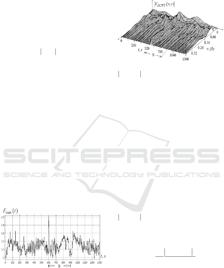
the analytical expression for CWT (7). The value
 
max
Ft
shown in Fig. 8 corresponds to the
maximum value of
 
,Vt
for each point in time
t
.
The function
 
max
Ft
varies in the range
 
max
0.4 2.5Hz F t Hz
.
The study of
 
max
Ft
during HDT (stage B,
600s
t
900s) shows the appearance of low-
frequency oscillations. The characteristic period
F
t
of such oscillations approximately equals
100
s. In
Fig.7 the graph for
 
n
RR t
shows two heartbeats at
the time
600t 
s separated by the interval
 
650
n
RR t 
ms. Therefore, at the same moment
600t 
s, the value of
 
max
Ft
1.54 Hz (Fig. 8).
Thus, for the frequency-modulated signal (17)
simulation, we can calculate the maximum local
frequency
 
max
Ft
at any time
t
.
Another wavelet transform applied to
 
max
Ft
(double continuous wavelet transform
DCWT [9]) makes it possible to study transients in the
variation of frequency. Applying double continuous
wavelet transform to the signal
 
max
Ft
allows us to
detect both aperiodic and oscillatory movements of
the local frequency relative to the trend.
Figure 8: Dependence
 
max
Ft
on time
()t ms
.
Fig.9 displays the result of DCWT with the
procedure of STS, which shows a sharp change in the
spectral structure of the signal at stage B.
Figure 9: Dependence of double wavelet transform
 
DCWT
Vt
on frequency
()Hz
and time
()t ms
.
Fig. 9 shows that the tachogram is an alternation
of bursts of spectral activity in different spectral
ranges:
ULF = (
min
;0.015 
Hz); (VLF = (0.015; 0.04 Hz);
LF = (0.04; 0.15 Hz); HF =(0.15; 0.4 Hz).
The value of
min

is determined by the equation
(16), with the number of periods
5n 
,
2
x

.
To analyze heart tachogram during nonstationary
functional tests, we introduced quantitative
characteristics describing the dynamics of changes in
spectral properties of the signal
 
max
Ft
. Such
characteristics are the instantaneous spectral integrals
 
Et

, and the mean values of the spectral integrals
 
ES


at the stages
 
,,S A B C
in different
spectral ranges
 
, ; ;ULF VLF LF HF
.
To study the appearance and disappearance of
low-frequency oscillations
 
max
Ft
, we can calculate
the skeletons of DCWT showing the extreme line of
 
DCWT
Vt
on the plane

and
t
. The value
 
,t 
illustrates instantaneous frequency
distribution of the signal energy (local density of
energy spectrum of the signal)
 
 
2
,
2
,
DCWT
Vt
t
C





(18)
The constant
C

for the Morlet mother wavelet
(8) is approximately 1.013 (
1m 
). The dynamics of
time variation for different frequencies is determined
by spectral integral
 
Et

:
BIOSIGNALS 2019 - 12th International Conference on Bio-inspired Systems and Signal Processing
28

   
/2
/2
1
,E t t d





  






(19)
Spectral integral
 
Et

represents the average
value of the local density of the signal energy
spectrum integrated over a certain frequency range
[ / 2; / 2]

         
, where


denotes the middle of the interval,
 
– its width.
The time-variation of
 
Et

performs a kind of
signal filtration summing the contributions from
the local density of the spectrum
 
,t 
only in a
certain range of frequencies

={ULF, VLF, LF,
HF}. By studying DCWT of the signal and
calculating
 
Et

in

-range one can follow the
dynamics of appearance and disappearance of low-
frequency spectral components
 
max
Ft
.
The quantitative characteristics that describe the
average dynamics of the spectral properties of a
tachogram during nonstationary test have average
values of the spectral integrals at the stages
S={A,B,C} in the ranges μ. Assuming that stage S
starts at
 
I
tS
and ends at
 
F
tS
, the average
spectral integrals are equal at stage S and are
 
   
 
 
 
1
.
F
I
tS
FI
tS
E S E t dt
t S t S

 
  


(20)
We introduce the function
 
 
 
Et
dt
EA





,
(21)
which shows the instantaneous value of the spectral
integral in

range at the arbitrary time point
t
as
compared to its average value at rest (Stage A). In
addition, we introduce the function
 
/
dt

:
 
   
   
/
E t E A
dt
E t E A






,
(22)
which shows how the instantaneous ratio
   
/E t E t

varies over the ratio of average
spectral integrals
   
/E A E A

   
calculated at the stage of rest (Stage A). The functions
 
dt

and
 
/
dt

represent the variation of
spectral characteristics during the total tachogram
period as compared with the respective average
values observed at Stage A (

={ULF, VLF, LF,
HF};

={ULF, VLF, LF, HF} )
We determine the heart rhythm assimilation
coefficient in the spectral range

as
 
 
 
/
EB
D B A
EA






.
(23)
It reports the fold increase in the average spectral
integral
 
EB


for the

-range at Stage B
relative to the average value
 
EA


of spectral
integral for the same

-range at rest (Stage A).
The detailed calculations of
 
Et

and
 
ES


are given in (Bozhokin and Suslova,
2013), (Bozhokin et al., 2017). Fig. 10-13 represent
the results of DCWT analysis of nonstationary heart
rhythm using the STS technique.
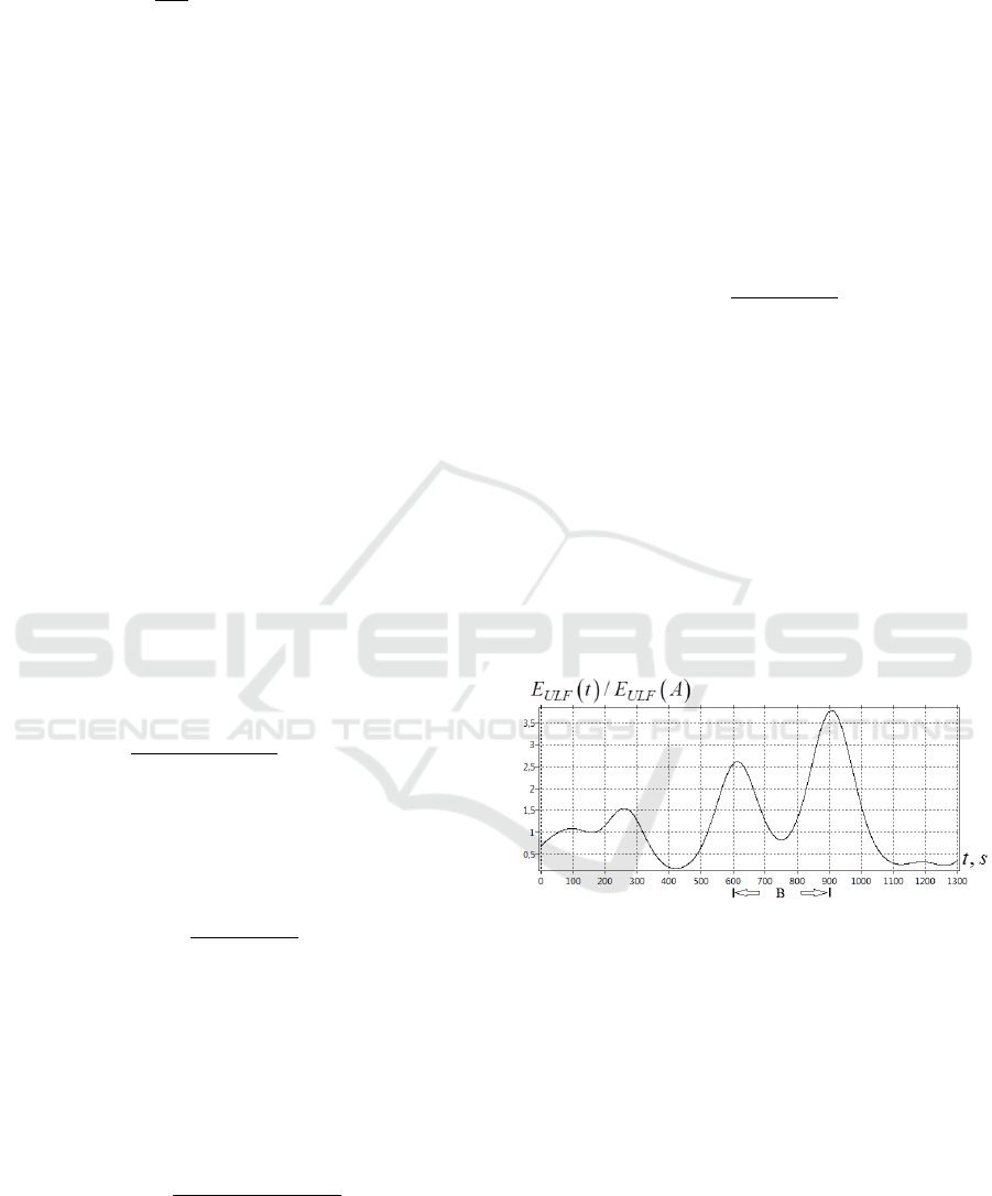
Figure 10: Spectral interval
 
ULF
Et
divided by the
average value in the stage A
 
ULF
EA
.
Fig.10 gives the plot of time behavior for
 
ULF
dt
(21). The heart rhythm assimilation
coefficient
 
/
ULF
D B A
(23) in the
ULF  
spectral range is 1.92. The coefficient
 
ULF
dt
(21)
reaches the maximal value
3.8
at
900t 
s. This
means that the instantaneous value of
 
ULF
Et
at
Stage B (test phase) is approximately 3.8 times
greater than the average value of
 
ULF
EA
at Stage
A (at rest). In this spectral range (ULF) during the
Elimination of Boundary Effects at the Numerical Implementation of Continuous Wavelet Transform to Nonstationary Biomedical Signals
29

time period
600 900t
s a strong trend in
 
max
Ft
is noticeable (Fig.8).
After the completion of HDT (
900t 
s), there
occurs a slow relaxation of the heart rate to the
equilibrium state, which takes about 300 s. The
characteristic time of frequency changes is equal to
100 s.
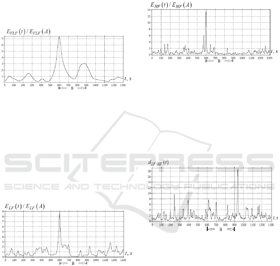
Figure 11: Spectral integral
 
VLF
Et
divided by its
average value
 
VLF
EA
at the stage A.
Fig.11 shows the behavior of
 
VLF
dt
(21). The
heart rhythm assimilation coefficient
 
/
VLF
D B A
in the
VLF  
spectral range equals
2.32
(23).
The maximum of
 
7.4
ULF
dt
(21) takes place at
600t 
s. Fig.11 shows rapid VLF rhythm activation
at Stage B (
600 900t
s) in comparison to Stage
A (
0 600t
s).
Figure 12: Spectral interval
 
LF
Et
divided by its
average value
 
VLF
EA
at the stage A.
Fig.12 represents the coefficient
 
LF
dt
as a
function of time. Note that at Stage B in the range
LF  
, the rhythm is also noticeably higher than at
stage A. The heart rhythm assimilation coefficient
 
/ 1.15
LF
D B A 
. Considering the oscillatory
motion of the maximal frequency
 
max
Ft
, we detect
flashes of vibrational activity in this spectral range LF
= (0.04; 0.15 Hz). For such flashes, the magnitudes of
spectral integrals can many times exceed the
background signal activity.
Figure 13: Spectral interval
 
HF
Et
divided by its
average value
 
HF
EA
at the stage A .
In the range HF = (0.15; 0.4 Hz), we can also
observe short flashes of activity in spectral integrals.
The maximum of
 
HF
dt
is approximately 14 times
greater than the background, but
 
/ 0.67
HF
D B A 
. This means that the average
activity at Stage B is less than the average activity at Stage
A.
Figure 14: Temporal dependence of
 
/LF HF
dt
.
Fig.14 demonstrates the temporal behavior of
 
/LF HF
dt
, which characterizes the instantaneous
ratio of
   
/
LF HF
E t E t
to the average value
   
/
LF HF
E A E A   
calculated at stage A.
The graph shows that at some time points the
instantaneous value
 
/LF HF
dt
becomes
significantly large. This indicates the moments of
tension in the physiological state of the patient and
can be used for diagnostic purposes.
BIOSIGNALS 2019 - 12th International Conference on Bio-inspired Systems and Signal Processing
30

4 CONCLUSION
The algorithm developed in the article, which allows
eliminating boundary effects in the numerical
implementation of CWT, becomes especially
important in the case of signals with the predominant
influence of low frequencies, when the observation
period for such signals is not too large. If the signal
shows significant variations, the information on the
behavior of the signal at the initial and final
observation stages becomes very important for the
correct conclusion about its amplitude-frequency
properties.
We believe that as biological signals are strongly
nonstationary, special technique is necessary to detect
variations in frequency and temporal structure. Using
CWT and DCWT with the STS procedure of boundary
effect correction helps to solve the problem. The
effectiveness of the technique is demonstrated in
application to the record of human heart tachogram
during functional test (HDT – head down).
The calculations were made based on the frequency-
modulated tachogram model proposed by the authors.
The technique of double continuous wavelet
transformation leads to the conclusion that
nonstationary tachogram can be represented as a
combination of activity flashes in different spectral
ranges. Such flashes may appear and disappear at
certain points in time and in different spectral ranges.
The quantitative characteristics of nonstationary
tachogram estimate the increased heart activity in the
period of changing the position of the body during the
HDT.
The method of studying the restructuring spectral
activity in the cardiac rhythm during the transitional
processes, which is suggested in this article, makes it
possible to reveal the dynamics of interaction
between parasympathetic and sympathetic parts of
the human autonomic nervous system. The proposed
quantitative parameters allow us to get an objective
assessment of the adaptive capabilities of the human
organism during various physical, orthostatic,
respiratory, psycho-emotional and medicated tests.
The proposed techniques help to reveal and
analyze important information, which can be used in
diagnostics.
ACKNOWLEDGMENTS
The work has been supported by the Russian Science
Foundation (Grant of the RSF 17-12-01085).
REFERENCES
Addison, P.S. (2017) The illustrated wavelet transform
handbook. Introductory theory and application in
Science, engineering, medicine and finance. Second
Edition, CPC Press.
Advances in Wavelet Theory and Their Applications in
Engineering, Physics and Technology. (2012). Edited
by Dumitru Baleanu.
Anderson, R., Jonsson, P., Sandsten, M. (2018). Effects of
Age, BMI, Anxiety and Stress on the Parameters of a
Stochastic Model for Heart Rate Variability Including
Respiratory Information, Proc. of the 11th
International Joint Conference on Biomedical
Engineering Systems and Technologies (BIOSTEC
2018), 4: BIOSIGNALS, P. 17-25.
Andreev, D.A., Bozhokin, S.V., Venevtsev, I.D.,
Zhunusov, K.T. (2014). Gabor transform and
continuous wavelet transform for model pulsed signals.
Technical Physics, 59(10):1428-1433.
Baevskii, R.M., Ivanov, G.G., Chireikin, L.V., et. al.,
(2002). Analysis of heart rate variability using different
cardiological systems: methodological
recommendations. Vestn. Aritmol., N.24: 65-91.
Bhavsar, R., Daveya, N., Sun,Y., Helian, N., (2018). An
Investigation of How Wavelet Transform Can Affect
the Correlation Performance of Biomedical Signals.
Proc. of the 11th International Joint Conference on
Biomedical Engineering Systems and Technologies
(BIOSTEC 2018). V. 4: BIOSIGNALS, P. 139-146.
Boltezar, M., Slavic, J., (2004). Enhancements to the
continuous wavelet transform for damping
identification on short signals. Mechanical systems and
signal processing, 18: 1065-1076.
Bozhokin, S.V., (2012). Continuous Wavelet Transform
and Exactly solvable Model of Nonstationary Signals.
Technical Physics, 57(7): 900-906.
Bozhokin, S.V., Suslova, I.M., (2013). Double Wavelet
Transform of Frequency-Modulated Nonstationary
Signal. Technical Physics, 58(12):1730-1736.
Bozhokin, S.V. Suslova, I.B., (2014). Analysis of non-
stationary HRV as a frequency modulated signal by
double continuous wavelet transformation method.
Biomedical Signal Processing and Control. 10: 34-40.
Bozhokin S.V., Suslova I.B., (2015). Wavelet-based
analysis of spectral rearrangements of EEG patterns and
of non-stationary correlations. Physica A. 421: 151–
160.
Bozhokin, S.V., Zharko, S.V., Larionov, N.V., Litvinov,
A.N., Sokolov, I.M. (2017). Wavelet Correlation of
Nonstationary Signals. Technical Physics, 62(6):837-
845.
Bozhokin, S.V., Lesova, E.M., Samoilov, V.O., Tarakanov
D.E., (2018). Nonstationary heart rate variability in
respiratory tests. Human Physiology, 44(1):49-57.
Cazelles, B, Chavex, M., Berteaux, D., Menard, F., Vik,
J.O., Jenouvrier, S., Stenseth, N.C. (2008). Wavelet
analysis of ecological time series. Oecologia,156:297-
304.
Elimination of Boundary Effects at the Numerical Implementation of Continuous Wavelet Transform to Nonstationary Biomedical Signals
31

Chui, C.K., Jiang O., (2013). Applied Mathematics. Data
Compression, Spectral Methods, Fourier Analysis,
Wavelets and Applications. Mathematics Textbooks for
Science and Engineering, v.2, Atlantis Press.
Cohen A., (2003). Numerical Analysis of Wavelet
Method.,North-Holland, Elsevier Science.
Ducla-Soares, J.L., Santos-Bento, M., Laranjo, S.,et al.,
(2007).Wavelet analysis of autonomic outflow of
normal subjects on head-up tilt, cold pressor test,
Valsalva manoeuvre and deep breathing. Exp. Physiol.
92(4): 677-686.
Hammad, M., Maher, A., Adil, K., Jiang, F., Wang, K.,
(2018). Detection of Abnormal Heart Conditions from
the Analysis of ECG Signals. Proc. of the 11th
International Joint Conference on Biomedical
Engineering Systems and Technologies (BIOSTEC
2018). V. 4: BIOSIGNALS, P. 240-247.
Hramov, A.E., Koronovskii, A.A., Makarov, V.A., Pavlov,
A.N., Sitnikova, E., (2015). Wavelets in neuroscience,
Springer Series in Synergetics, Springer-Verlag, Berlin,
Heidelberg.
Keissar, K., Davrath, L.R., and Akselrod, S. (2009).
Coherence analysis between respiration and heart rate
variability using continuous wavelet transform. Philos.
Trans. R. Soc., A. 367(1892):1393-1406.
Mallat, S., (2008). A Wavelet Tour of Signal Processing,
3rd ed., Academic Press, New York.
Podtaev S., Morozov M., Frick P., (2008). Wavelet-based
corrections of skin temperature and blood flow
oscillations. Cardiovascular Engineering, 8(3):185-
189.
Tankanag, A.V., Chemeris, N.K., (2009). Adaptive wavelet
analysis of oscillations in the Human peripherical blood
flow. Biophysics, 4(3):375-380.
Ulker-Kaustell, M., Karoumi, R. (2011). Application of the
continuous wavelet transform on the free vibration of a
steel-concrete composite railway bridge. Engineering
structures, 33: 911-919.
Wavelets in Physics, (2004). Edited by J.C. Van.den Berg,
Cambridge University Press.
BIOSIGNALS 2019 - 12th International Conference on Bio-inspired Systems and Signal Processing
32