Classification of Ground Moving Radar Targets with RBF Neural
Networks
Eran Notkin
1
, Tomer Cohen
1
and Akiva Novoselsky
2
1
Department of Electrical and Computer Engineering, Ben-Gurion University of the Negev Beer Sheva, Israel
2
ELTA Systems Ltd. Group and Subsidiary of IAI Ltd Ashdod, 7710202, Israel
Keywords:
GMTI, RBF Neural Network, Radar Target Classification, SNR, RCS.
Abstract:
This paper presents a novel method for classification of targets detected by Ground Moving Target Indication
(GMTI) radar systems. GMTI radar systems provide no direct information regarding the type or size of the
detected targets. The suggested method allow classification of ground moving targets into few groups of size,
by analysis of Signal to Noise Ratio (SNR) values of GMTI radar measurements. The classification method is
based on Radial Basis Function (RBF) neural networks. The data used as features for classification composed
of Radar Cross Section (RCS) values of the target (obtained from the SNR values) in varying aspect angles.
The proposed classifier was tested on diverse simulative cases and yielded very good results in classification
of targets for three groups of size.
1 INTRODUCTION
Target classification for a GMTI radar system is a
challenging task due to the lack of any informa-
tion regarding the target’s spatial size or shape in
the radar’s raw data (Blackman and Popoli, 1991)–
(Skolnik, 1962). On the other hand, such a feature
is vital due to the growing need to provide indica-
tion regarding the type of detected radar targets when
no optical sensors are available. Therefore, for the
past decades many researches turned their effort to
introduce a method for estimating the size of the tar-
gets from the radar raw data (Vespe, 2007)–(Zhao and
Bao, 1996).
Vespe, in his Ph.D. thesis (Vespe, 2007), gives
a survey of the methods developed for GMTI target
classification. The author describes three fundamen-
tals classification methodologies. The first methodol-
ogy relay on a database of previously collected mea-
surements to form a library of templates (a series of
class-labeled patterns). Classification of a new target
is based on comparison of the pattern formed by the
target’s measurements, and the patterns in database.
However, it can be very difficult to obtain enough
measurements to construct a reliable database. The
second methodology relays on Computer Aided De-
sign (CAD) target models, and computational predic-
tion of targets’ radar measurements or features. The
possibility of modeling any target class having any
possible configuration is the principal advantage of
this method, counterbalanced by the difficulty of ob-
taining reliable simulated measurements. The third
method relays on a priori knowledge of the target’s
physical and electrical characteristics, offering the ad-
vantage of classification which does not require radar
measurements to represent the target class.
The following paragraphs describe methods for
radar target classification based on the RCS signature
of targets(Register et al., 2008), (Backes and Smith,
2013), (Lee et al., 2016).RCS signature of a target is
the RCS value measured in every given orientation of
the target. The orientation of the target is determined
by the aspect angle, i.e. the angle between the radar’s
Line of Sight (LOS) and the target’s velocity direc-
tion. RCS values are not obtained directly from the
radar measurements, but extracted from the SNR of
radar measurements using the radar equation (Skol-
nik, 1962).
The work of A. Register et al. (Register et al.,
2008), use RCS measurements as a feature for tar-
get classification. The authors aim to classify radar
targets by associating the detected target to one of
two types, a reentry vehicle (RV) and a tank. The
classification is performed by a decentralized fusion
algorithm which is provided with results from Lo-
cal Decision Functions (LDFs). The LDFs provide
a decision regarding the targets identity, based on the
RCS characteristics of the target. The RCS values are
328
Notkin, E., Cohen, T. and Novoselsky, A.
Classification of Ground Moving Radar Targets with RBF Neural Networks.
DOI: 10.5220/0007254203280333
In Proceedings of the 8th International Conference on Pattern Recognition Applications and Methods (ICPRAM 2019), pages 328-333
ISBN: 978-989-758-351-3
Copyright
c
 2019 by SCITEPRESS – Science and Technology Publications, Lda. All rights reserved

extracted from SNR measurements, measured across
multiple dwells. The classifier was tested on simula-
tions of X-band radar observing an RV and a tank. In
some cases, the LDFs showed unstable classification
results. However, the fusion algorithm was found ef-
ficient and manage to replace false decisions of the
LDFs.
T. Backes and L. D. Smith (Backes and Smith,
2013) attempt to improve RCS estimation by data
censoring methods. The authors refer to two different
methods for data censoring. In the first method, the
data is censored through the removal of values that
cross a certain maximum or minimum threshold. In
the second method, the data is censored by removing
a fixed quantity of peripheral samples. For target clas-
sification, the authors use a Maximum Likelihood Es-
timator (MLE) based on Swerling III and IV distribu-
tion models of mean RCS. The paper provides a com-
parison between the error biases of conventional, un-
censored MLE and censored MLE using the first cen-
soring method. The classification results show that
censored MLE performance substantially exceeds the
performance of the conventional MLE.
S. Lee et al. (Lee et al., 2016) present a method
to design a fuzzy classifier to classify shell-shaped
targets. The classification is based on RCS mea-
surements with consideration of the aspect angle and
polarization dependencies in various flight scenarios.
The fuzzy classifier consists of membership functions
(MFs) which relate the RCS value to the probability
that the input belongs to each specific target class.
The authors suggest three different MFs Gaussian,
trapezoidal, and triangle MF. Particle Swarm Opti-
mization (PSO) is applied to optimize MF parame-
ters, to maximize classification capabilities. PSO is a
stochastic search method, effective in optimizing dif-
ficult multidimensional problems. The classifier was
tested in simulative environment. The best perfor-
mance was given by Gaussian fuzzy, achieving 75%
hit-rate.
The works mentioned above do not present a
comprehensive general method for classifying ground
moving radar targets. The reason is that SNR values
are characterized by large variances, and thus samples
of targets from different classes overlap each other. In
addition, the reflected signal’s SNR values are very
sensitive to changes in aspect angle (the angle be-
tween the intrinsic wave direction and the target’s ori-
entation). Even a slight change in aspect angle can
cause fluctuations of 20 dBsm, in SNR values (Skol-
nik, 1962).
This paper presents a new method for classifying
the GMTI radar targets based on Radial Basis Func-
tions (RBF) neural networks (Bishop et al., 1995) us-
ing RCS measurements with consideration of the as-
pect angle. RBF neural networks provide non-linear
classification and robust performance in classification
of data characterized by large variances, when the
classification is only into several classes. Containing
only one hidden layer, these networks offer the advan-
tage of short training time, fast classification, and rel-
atively simple implementation. Considering the char-
acteristics of the raw data provided by GMTI radar
measurements, and the low number of classes, this
type of networks was found suitable for achieving our
goal.
RBF networks for classifying targets have already
been used in some previous works (Guosui et al.,
1996)–(Zhao and Bao, 1996). L. Guosui et al. (Gu-
osui et al., 1996), used modified RBF networks for
classifying between moving targets of man, bicycle
and truck. Unlike our work, the data used for classi-
fication was Doppler frequency spectrum of the radar
measurements. In addition, the classifier presented in
the current work is restricted to classification of mo-
torized vehicles alone to classes that possess much
less distinctive characteristics. Also, the work of Q.
Zhao and Z. Bao (Zhao and Bao, 1996) was restricted
to 3 different military aircrafts, and does not introduce
the ability to classify ground moving targets.
This paper is organized as follows. Section 2 pro-
vides a general introduction to Neural Networks and
the RBF network. Section 3 presents the implemen-
tation of RBF network for GMTI radar target classifi-
cation. Section 4 describes the simulations and result.
Finally, in Section 5 we present the conclusions of this
work.
2 NEURAL NETWORKS AND
RBF NETWORK
This section is composed of two subsections. The first
subsection provides a general background on the topic
of artificial networks. The second subsection concen-
trates on RBF neural networks.
2.1 Neural Networks
Artificial neural networks are mathematical models
for data processing which are inspired by the struc-
ture of the mammal brain (Bishop et al., 1995). A
large artificial neural network might have hundreds or
thousands of processing units, while there are simpler
networks composing of tens of processing units. The
processing units are denoted as neurons. The neurons
are organized in layers. The first and last layers are
referred to as input and output layers, and in between
Classification of Ground Moving Radar Targets with RBF Neural Networks
329

there are one or more additional layers, which are re-
ferred to as hidden layers.
The use of neural networks involves feature ex-
traction. This means that we do not use all the data
regarding our classification problem, not in the train-
ing stage, nor in the activation of the network. To
reduce complexity, processing time, and enhance per-
formance, one must choose only certain features of
the subject for classification, which represent the sub-
ject/class in the best way, and will be the input of the
network.
Neural Networks (NN) based algorithms are used
to solve a variety of problems, such as speech recog-
nition, data mining, medical diagnosis, and computer
vision. Most importantly for the case of this paper,
NN based algorithms have been found very useful for
complex, nonlinear classification tasks. For the scope
of this work, supervised learning is especially rele-
vant, where the class of each target in the training
database is known, and used in the procedure of net-
work training.
2.2 RBF Networks
A Radial Basis Function, is a real valued function in
which the value is determined by the distance between
the input vector and the origin or a given center, i.e.
φ(x, c) = (
k
x − c
k
) (1)
where x is an input vector of dimension d and c is
the center vector of the same dimension. We can use
the RBF to approximate any given function y(x) as a
weighted sum over M basis functions.
y =
M
∑
i=1
ω
i
φ(
k
x − c
i
k
) (2)
where w
i
is the i
th
weighting coefficient and c
i
is
the appropriate center. It can be shown that any con-
tinuous function on a given interval can be interpo-
lated with arbitrary accuracy by this summation, for
sufficiently large number of M (Bishop et al., 1995).
The scalar equation 2, can be generalized to a mul-
tivariate equation of any dimension K, where each
component is given by such weighted sum.
y(k) =
M
∑
i=1
ω
ik
φ(
k
x − c
i
k
), k ∈ [1, . . . , K] (3)
Equation 3 can be represented as a neural network
as demonstrated in Fig.1. The RBF network is con-
structed from three basic layers: input, hidden, and
output. In Fig.1 the input is the vector x, the hidden
layer is constructed from the M functions φ(x), and
the output is constructed from K classes.
Figure 1: RBF network architecture: x = [x
1
, . . . , x
d
] is
the input vector- layer no. 1, φ
1
, . . . , φ
M
are the activation
functions-layer no. 2, W
11
, . . . , W
MK
are the weights, and
layer no. 3 is constructed of k output classes.
During classification procedure, the feature vector
is sent to each of the activation functions as an input.
Each of the activation functions provides a value cor-
responding to the features of the target, φ
i
(x). The
output of the hidden layer is an M dimensional acti-
vations vector.
Φ(x) = [φ
1
(x), ..., φ
M
(x)], Φ ∈ R
M
(4)
The final output of the RBF neural network is a
K dimensional vector y, obtained by a multiplication
of the activations vector by an optimized weights ma-
trix W (the optimized weights matrix is constructed
during the training procedure).
y = W ·Φ(x), W ∈ R
K×M
(5)
The component k of the vector y
y(k) =
M
∑
i=1
[W ]
k,i
φ
i
(x) (6)
is assigned to class k in the output layer. The value
of each component of the vector y represents the as-
signment score to the appropriate class. The class
with the highest compatibility score is the predicted
class.
ClassPrediction = argmax
k∈[1,2,...,K]
{y(k)} (7)
In advance of the classification procedure de-
scribed above, the network is trained using a database
containing measurements of known targets. In the
first step the measurements are divided into M clusters
by an unsupervised clustering algorithm. Then, the
weights between the hidden layer, and output layer,
(the components of the W matrix) are calculated by a
supervised training algorithm (Bishop et al., 1995).
ICPRAM 2019 - 8th International Conference on Pattern Recognition Applications and Methods
330

3 THE PROPOSED METHOD FOR
TARGET CLASSIFICATION
USING RBF NETWORKS
This section provides a description of the features
extraction procedure, and the implementation of the
RBF network, for GMTI radar targets classification.
The features we use are RCS values of the targets
at various aspect angles. In our simulations, the tar-
gets are assumed to be symmetrical with respect to
axes x and y. Therefore, every aspect angle can be
projected into the range of [0 − 90]. The aspect angles
are divided into 9 domains: [0, 10) ⊆ α
1
, [10, 20) ⊆
α
2
, [20, 30) ⊆ α
3
, etc.
When a target is detected, the radar system uses
a tracker to associate consecutive radar observations
(known as "plots") of the target into a track. Using
tracking information the direction of the target’s ve-
locity is obtained, and the aspect angle of the target in
each plot is calculated.
The RCS of the target is extracted from the SNR
value of each plot using the Radar equation (Skolnik,
1962). Each RCS value is assigned to the appropriate
element of the feature vector according to the aspect
angle of the target in the corresponding plot. When
few plots fall in the same angle domain, the average
RCS value of these plots is used. We note that the
choice of number of plots for classification introduces
a trade-off between accuracy and duration of the clas-
sification procedure: the more plots used for classifi-
cation; the more time is invested for collecting them.
In most cases, the target is not observed at all an-
gle domains, i.e. some of the elements in the feature
vector do not contain information. In these cases, the
value ’0’ is assigned to the regions with no available
information. The value ’0’ means no information re-
garding the target, rather than actual ’0’ value. There-
fore a weights vector is concatenated to the feature
vector, to ’mark’ the elements with no information.
The weights vector consists of the value ’100’ in el-
ements which correspond to regions that contain in-
formation, and the value ’0’ in all other cells. This
enables the network to adapt to those cases in which
the feature vector is partial, and enhances the versatil-
ity of the classifier.
For a given target, the feature vector corresponds
to a unique pattern of RCS values with respect to as-
pect angles. Using a substantial amount of these vec-
tors as a training set, we can train the network to rec-
ognize the typical pattern of each class, and in turn,
use it for classification when new unknown measure-
ments are acquired.
In the current work, the activation functions
{
φ
i
}
M
i=1
of the hidden layer are Gaussian functions
with expectancy µ
i
and the covariance matrix Σ
i
.
φ(x) = e
−
1
2
(x−µ
i
)
T
Σ
−1
i
(x−µ
i
)
(8)
The parameters of the activation functions and the
weights matrix are determined during training proce-
dure using a database of N observations
{
x
i
}
N
i=1
of
known targets
{
t
i
}
N
i=1
. Each target is labeled accord-
ing to its class. For example, a target of class k ∈
{
1, .., K
}
is labeled by the vector t
i
= [t
i1
, ..., t
iK
]
T
∈
R
K
, where t
i j
=

1, j = k
0, else
.
In the first stage of training, the training data
points are divided to M subsets by the k-means clus-
tering algorithm. The expectancies
{
µ
i
}
M
i=1
of the ac-
tivation functions are determined by the mean vec-
tors of the data points of in each subset. The covari-
ance matrices
{
Σ
i
}
M
i=1
are determined according to the
average square distance between the observations of
each subset and the mean vector of each subset.
In the second stage of training the values of the
weights, i.e. the elements of the weights’ matrix W,
are given by the solution of the following least squares
problem:
Minimize
W ∈R
K×M

(W · Ψ − T )
T
(W · Ψ − T )

Φ(x) = [φ
1
(x), ..., φ
M
(x)] , Φ ∈ R
M
Ψ = [Φ(x
1
), ..., Φ (x
N
)] , Ψ ∈ R
M×N
T = [t
1
, ..., t
k
] , T ∈ R
K×M
(9)
Where Φ is the activation vector, Ψ is the activa-
tion matrix and T is the target matrix. The solution of
the least squares problem is given by
W
T
= Ψ
†
· T (10)
4 SIMULATION & RESULTS
In this section, we introduce the simulated database,
and a performance analysis of the suggested classifier.
The database of radar plots is based on 14 tar-
get models which were designed per dimensions of
known vehicles (e.g. Mazda 3, Mercedes truck, Ford
pick-up truck, etc.). The observations are obtained in
many different GMTI simulated scenarios. We sim-
ulate a database which consists of 30,000 radar de-
tections. To test the classifier, the database is divided
into two parts: 70% of the data is used as training
data, and 30% is used as test data. The aspect angle
and the RCS value of each observation are calculated
as explained in section 3. In addition, since we are
working with simulated data, the ID number which
defines the identity of the detected target is known.
Classification of Ground Moving Radar Targets with RBF Neural Networks
331

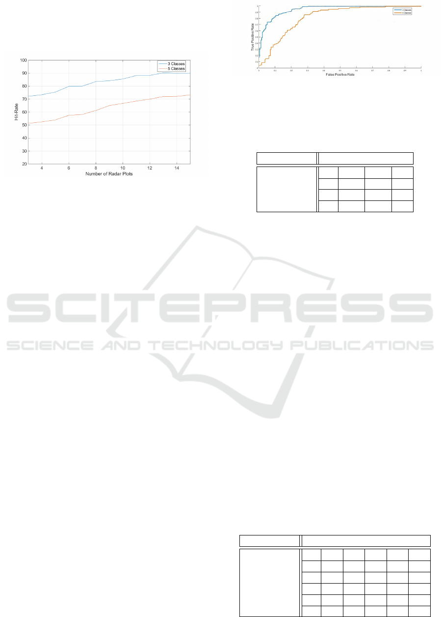
Fig.2 present a comparison between classifica-
tions as function of the numbers of radar plots. The
results refer to classification of targets to three and
five classes of size.
Figure 2: Classification hit rates for 3 and 5 classes as func-
tion of the number of radar plots used for classification.
As Fig.2 demonstrates, classification hit rates for
cases of few radar plots are low. As we take more
radar plots in consideration, the data obtained regard-
ing the target is more robust and allows for higher ac-
curacy in classification. The downside of classifica-
tion using many radar plots is the time consumed for
acquiring these plots. We found that using 10 radar
plots enables classification with good performance
for 3 classes, while increasing the number of plots
does not substantially enhances performance. In ad-
dition, Fig.2 shows that classification into five classes
of size results with an inferior performance compared
with classification into three classes of size, because it
needs to differentiate between more target types, and
hence it has more mis-classifications.
In Fig.3, we present the Receiver Operating Char-
acteristic (ROC) curves that show true positive classi-
fication rates versus true negative classifications rates.
Classification of middle-sized targets to the middle-
size class is considered a true positive classification.
Classification of other targets to the middle-size class
is considered a true negative. The curves relate to dis-
tinctions of targets to three or five classes. Choosing
between three- or five-classes distinctions introduces
the trade-off between achieving a more delicate dis-
tinction and achieving results with higher reliability.
In Table 1 and Table 2, the results are presented
by confusion matrices to demonstrate the classifiers
performances. The rows of each matrix represent the
actual class of the target, while the columns represent
the predicted class. In table the classes are arranged
by increasing size of vehicles. The first class (A) rep-
resents the smallest vehicles, and the last class repre-
sents the largest vehicles. From table 1 we can extract
that, for example, out of 152 true small vehicles, we
were correct in 123 vehicles and the other vehicles
Figure 3: ROC curves for distinction between three or five
classes. True positive means - classification of middle-size
targets to the middle-size class and classification of other
targets to the middle-size class is considered as true nega-
tive.
Table 1: Confusion Matrix for Three Classes Distinction.
Prdicted class
Actual class
A B C
A 123 29 0
B 12 159 5
C 0 9 71
were predicted as medium size. No vehicle was pre-
dicted as a large one.
In general, the confusion matrices provide indica-
tion of the classifier’s stability. The elements on the
matrix’s diagonal, which indicate correct classifica-
tion, have much greater values than the rest. Elements
which are located far from the matrix diagonal con-
tain small or zero values, indicating that most targets
which are miss-classified are usually classified to a
neighbor class. These results show that the RBF clas-
sifier rarely makes ’big’ mistakes such as classifying
a small target as a big target. The confusion matrices
also demonstrate the difficulty of classifying targets
to high number of classes. By looking at Table 2, we
can learn that distinction between class C, and class
D is challenging.
Fig.4 presents a comparison of the performance of
our classifier, with the results obtained by a Minimum
Mean Square Error (MMSE) criterion based classifi-
cation method. To perform classification based on the
MMSE criterion, we use the training dataset to create
an RCS-to-angle typical pattern for each class. The
pattern is created by averaging the RCS values taken
in every specific angle separately. Then for a given
unknown target, the mean square error between the
Table 2: Confusion Matrix for Five Classes Distinction.
Prdicted class
Actual class
A B C D E
A 48 5 2 1 0
B 9 50 17 4 0
C 3 7 48 20 2
D 0 3 34 39 4
E 0 1 2 3 74
ICPRAM 2019 - 8th International Conference on Pattern Recognition Applications and Methods
332

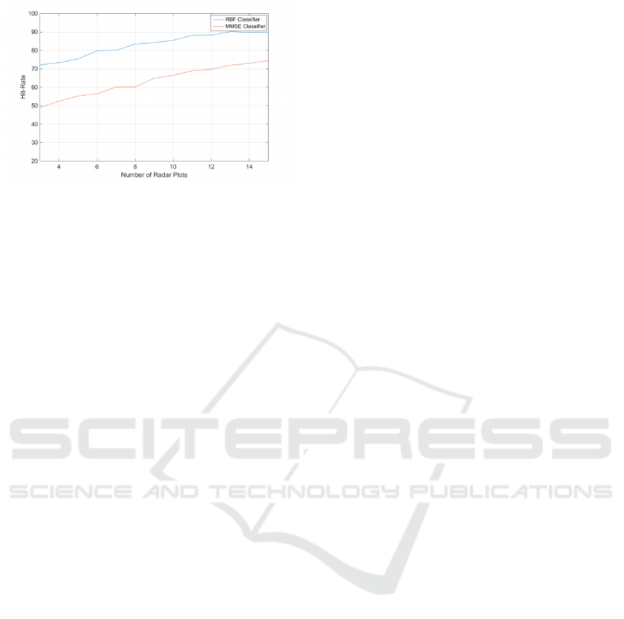
Figure 4: Comparison of the RBF network based classifier,
and an MMSE based classifier performances. Hit Rate as
Function of Measurements Number for classification to 3
Classes.
feature vector and the RCS-to-angle patterns of each
class is computed. The target is assigned to the class
with the minimum mean square error.
5 CONCLUSION
In this paper, a classifier for GMTI radar targets us-
ing RBF neural networks is proposed. The classifi-
cation is done based on a feature vector which con-
tains the RCS values in different observed aspect an-
gle regions of the target. The proposed solution can
also handle cases of insufficient data and classify tar-
get when the feature vector is not fully obtained. The
above attribute makes the classifier suitable for real-
time applications and offers added versatility. Com-
parison results have shown that our method is consid-
erably better than the MMSE classifier for the same
database. In addition, simulations have shown that
this approach is suitable for classifying ground mov-
ing radar targets into 3 classes of size, with up to 90%
hit-rate.
ACKNOWLEDGMENT
The authors would like to thank Gregory Lukovsky,
Nimrod Teneh, Nati Yannay and David Feldman for
useful discussions.
REFERENCES
Backes, T. and Smith, L. D. (2013). Improved rcs model
for censored swerling iii and iv target models. In
Aerospace Conference, 2013 IEEE, pages 1–4. IEEE.
Bishop, C., Bishop, C. M., et al. (1995). Neural Networks
for Pattern Recognition. Oxford University Press.
Blackman, S. and Popoli, R. (1991). Design and analysis of
modern tracking systems (artech house radar library.
Artech house.
Guosui, L., Yunhong, W., Chunling, Y., and Dequan, Z.
(1996). Radar target classification based on radial
basis function and modified radial basis function net-
works. In Procceedings of CIE International Confer-
ence of Radar, 1996., pages 208–211. IEEE.
Lee, S.-J., Jeong, S.-J., Kang, B.-S., Kim, H., Chon, S.-
M., Na, H.-G., and Kim, K.-T. (2016). Classifica-
tion of shell-shaped targets using rcs and fuzzy clas-
sifier. IEEE Transactions on Antennas and Propaga-
tion, 64(4):1434–1443.
Register, A., Blair, W., Ehrman, L., and Willett, P. K.
(2008). Using measured rcs in a serial, decentral-
ized fusion approach to radar-target classification. In
Aerospace Conference, 2008 IEEE, pages 1–8.
Skolnik, M. I. (1962). Introduction to Radar Systems.
McGraw-Hill.
Vespe, M. (2007). Multi-Perspective Radar Target Classifi-
cation. PhD thesis, Univercity of London.
Zhao, Q. and Bao, Z. (1996). Radar target recognition using
a radial basis function neural network. Neural Net-
works, 9(4):709–720.
Classification of Ground Moving Radar Targets with RBF Neural Networks
333