Bootstrapping Vector Fields

Paula Ceccon Ribeiro and H

elio Lopes

Pontif

ıcia Universidade Cat

olica do Rio de Janeiro, Departamento de Inform

atica, Rio de Janeiro, Brazil

Keywords:

Vector Field, Uncertainty Quantiﬁcation, Helmholtz-Hodge Decomposition, Bootstrapping.

Abstract:

Vector ﬁelds play an essential role in a large range of scientiﬁc applications. They are commonly generated

through computer simulations. Such simulations may be a costly process since they usually require high

computational time. When researchers want to quantify the uncertainty in such kind of applications, usually

an ensemble of vector ﬁelds realizations are generated, making the process much more expensive. In this

work, we propose the use of the Bootstrap technique jointly with the Helmholtz-Hodge Decomposition as

a tool for stochastic generation of vector ﬁelds. Results show that this technique is capable of generating a

variety of realizations that can be used to quantify the uncertainty in applications that use vector ﬁelds as an

input.

1 INTRODUCTION

It is recognized in the literature that the task of model-

ing a physical spatial/temporal phenomenon is a very

important for decision making applications (Beccali

et al., 2003). When you have to deal speciﬁcally on

the natural phenonema forecasting, it is mandatory to

represent uncertainty (Mariethoz and Caers, 2014).

Several physical phenomena models that consider

uncertainty have two categories: 1) deterministic

models, which generates physically-based simulated

outcomes; 2) stochastic models, which provides re-

alizations that somehow cover the uncertainty space

and at the same time mimic the physics (providing a

certain level of realism) (Mariethoz and Caers, 2014).

The main objective of this paper is to present a

new stochastic method to generate 2D vector ﬁelds,

since they are very important in a variety set of de-

cision making problems related to Scientiﬁc Comput-

ing. Applications that make use of vector ﬁelds in-

clude, for example: ﬂuid ﬂow simulation (Anderson

and Wendt, 1995), analysis of MRI data for medical

prognosis (Tong et al., 2003) and weather prediction

(Luo et al., 2012), just to cite a few. The deterministic

simulation of vector ﬁelds in such applications may

require expensive numerical computations (Anderson

and Wendt, 1995). The stochastic generation of phys-

ically realistic vector ﬁelds realizations is a challeng-

ing task. Many algorithms for multivariate stochas-

tic simulation are based on very complex probabilistic

models (Popescu et al., 1998; Xiu, 2009; Lall et al.,

2016) and generally they are not adequate to mimic

physical phenomena such as wind, for example.

In this work, we propose an algorithm to stochas-

tically simulate vector ﬁeld realizations based on a

given gridded 2D vector ﬁeld V, which will from

now on be called the training data. Such algo-

rithm is based on the Helmholtz-Hodge Decompo-

sition (HHD) (Bhatia et al., 2013) and on the non-

parametric Bootstrap method (Efron, 1979). The pro-

posed algorithm aims to physically mimic V and ap-

propriately cover the space of uncertainty. More pre-

cisely, our algorithm ﬁrst use the HHD of V to ob-

tain its rotational-free and divergence-free potentials

components. With such potentials in hand, we per-

form a bootstrap-like approach to generate R other re-

alizations of these potentials and differentiate them.

Finally, we add the generated components to the

original harmonic component to generate R vector

ﬁeld realizations. Through Multi-Dimension Scaling

(MDS), we could verify that our results were capable

to provide some variability. To exemplify its use, we

apply our algorithm to the uncertainty quantiﬁcation

introduced by the use of the curl and the divergence

ﬁnite-difference differential operators.

Paper Outline. The remainder of this paper is or-

ganized as follows: Section 2 presents some previous

and related work. Section 3 and 4 describes the Boot-

strap method and the Helmholtz-Hodge Decomposi-

tion, in that other. Section 6 presents an analyses of

the method’s capabilities, whilst Section 7 shows an

application of the technique, followed by the perfor-

Ribeiro, P. and Lopes, H.

Bootstrapping Vector Fields.

DOI: 10.5220/0007248900190030

In Proceedings of the 14th International Joint Conference on Computer Vision, Imaging and Computer Graphics Theory and Applications (VISIGRAPP 2019), pages 19-30

ISBN: 978-989-758-354-4

mance results in Section 8. Finally, Section 9 presents

our conclusion as well as some ﬁnal remarks and fu-

ture studies.

2 RELATED WORK

This section has the objective to discuss the related

work about the three main concepts used in this work:

stochastic simulation, Helmholtz-Hodge Decomposi-

tion and the Bootstrap method.

Stochastic Simulation. As mentioned in the previ-

ous section, the stochastic generation of physically

realistic vector ﬁelds realizations is a challenging

task. In one side, many algorithms based on proba-

bilistic models for multivariate stochastic simulation

(Popescu et al., 1998; Xiu, 2009; Lall et al., 2016)

are very complex mathematically speaking and gen-

erally they are not adequate to mimic physical phe-

nomena such as wind, for example. In the other side,

there are several geostatistical methods in the litera-

ture dedicated to the stochastic simulation of spatial

physical phenomena (Lantu

ejoul, 2013). Generally,

they are applied to the generation of univariate con-

tinuous or categorical functions deﬁned on a 2D or

3D grid. They usually propose a parametric model

of uncertainty to formulate the lack of knowledge,

and models based on variogram are the most tradi-

tional ones (Oliver and Webster, 2014). Alternatively,

non-parametric approaches, such as the ones based on

Multiple-Point Statistics (MPS), have received a lot of

investigation in the last ﬁve years. These approaches

generate realizations of a spatial phenomenon based

on a training image, which implicitly describes the

phenomenon’s construction process (Mariethoz and

Caers, 2014). These methods have a very strong

connection with computer graphics’ texture synthe-

sis techniques (Mariethoz and Lefebvre, 2014), like

Image Quilting (Efros and Freeman, 2001), for exam-

ple. Similarly to MPS methods, this work proposes a

new non-parametric method for the stochastic genera-

tion of 2D vector-ﬁelds that is also based on a training

data. However, this new method uses the bootstrap

technique instead of the MPS.

Helmholtz-Hodge Decomposition. A wide range

of the applications of the Helmholtz-Hodge Decom-

position can be found in the literature. These include

the use of the HHD to detect singularities for ﬁnger-

print matching (Gao et al., 2010), its application in the

ﬁeld of complex ocean ﬂow visualization and anal-

ysis for feature extraction (Wang and Deng, 2014),

cardiac video analysis (Guo et al., 2006), hurricane

eye tracking (Palit, 2005) and the aerodynamic design

of cars and aircrafts (Tong et al., 2003). Recently,

Ribeiro and Lopes (Ribeiro et al., 2016) proposed the

use of the HHD as a tool to analyze 2D vector ﬁeld

ensembles. This work will use the HHD to decom-

pose the training data in order to obtain the rotational-

free and the divergent-free potentials. With these two

scalar ﬁelds in hands a bootstrap-based perturbation is

performed and the resulted ﬁelds are then differenti-

ated to construct a vector ﬁeld realization by summing

their perturbed components. Perturbing the scalar po-

tentials independently is fundamental to achieve the

objective of providing a certain level of realism of the

generated vector ﬁelds.

Bootstrap. The Bootstrap method is a statistical

method based on resampling with replacement. It is

commonly applied to measure the accuracy of statis-

tical estimators (Efron, 1979). In general, such accu-

racy could be deﬁned in terms of bias, variance, conﬁ-

dence intervals, prediction error or some other disper-

sion measure. This technique has been applied to vi-

sual computing problems, such as: performance eval-

uation for computer vision systems (Cho et al., 1997),

searching for radial basis function parameter (Liew

et al., 2016), evaluation of the inﬂuence of hidden

information on supervised learning problems (Wang

et al., 2014) and edge detection (Fu et al., 2012),

among others. This technique has in also very impor-

tant in this paper. Not only because it performs the

perturbation of the potential ﬁelds, but also because it

is adopted to quantify the algorithm uncertainty intro-

duced by the use of the curl and the divergence ﬁnite-

difference differential operators.

3 THE BOOTSTRAP METHOD

The Bootstrap method is based on the notion of a

bootstrap sample (Efron, 1979; Wasserman, 2004).

To better understand it, let

F be an empirical distribu-

tion, with probability 1/n on each of the n observed

values x

, with i ∈ {1,2,··· ,n}. Then, a bootstrap

sample is deﬁned as a random sample of size n drawn

from

F with replacement, say x

∗

= (x

∗

,··· , x

∗

) .

The star notation indicates that x

∗

is not the actual

data set x, but a randomized, or resampled, version of

x. For more details about this technique, see (Wasser-

man, 2004).

With this concept in mind, assume that

= g(x

,···x

) is a statistic of the data set

,··· , x

}. To compute the variance of T

, denoted

by V

), it would be necessary to know the

distribution F of the data. Often, however, this

GRAPP 2019 - 14th International Conference on Computer Graphics Theory and Applications

is unknown. The Bootstrap technique estimates

) by the use of stochastic simulations, where

the unknown distribution F is approximated by a

distribution named

F. Then, an approximation of

) is computed as V

). Generating B boot-

strap samples, it is now possible to approximate the

distribution of T

by evaluating T

∗

= g(x

∗

,··· , x

∗

Using this distribution, we can ﬁnally compute the

variance V

) according to the following formula:

) =

∑

i=1

∗

−

∑

b=1

∗

n,b

, (1)

where T

∗

, i = 1,.. .,B, represents the statistics com-

puted at the i

bootstrap sample.

4 HELMHOLTZ-HODGE

DECOMPOSITION

The Helmholtz-Hodge Decomposition (Chorin and

Marsden, 1993) states that a square-integrable vector

ﬁeld V can be formulated as the sum of three orthog-

onal components:

V = ∇ϕ + ∇ ×ψ + h, (2)

where ∇ϕ is the rotational-free term (∇ ×∇ϕ = 0),

∇ ×ψ is the divergence-free term (∇ ·(∇ ×ψ) = 0)

and h is the harmonic term (∇×h = 0 and ∇ ·h = 0).

Figure 1 shows an example.

The scalar ﬁeld ϕ is called the potential ﬁeld of

the curl-free term.

The curl of a 2D vector ﬁeld V is deﬁned by

∇ ×V = ∇ ×(V

) =



∂V

∂x

−

∂V

∂y



Thus, one can write ∇ ×V as (∇ ·J)V, where J is

an operator that rotates a vector by

in a clockwise

direction: J(x,y) = (y, −x).

As a consequence, Equation 2 can be rewritten for

a 2D vector ﬁeld (Polthier and Preuß, 2003) as:

V = ∇ϕ + J(∇ψ) + h, (3)

where ψ is a scalar ﬁeld that will be called the poten-

tial ﬁeld of the divergent-free component.

To obtain the HHD of a given 2D vector ﬁeld V

means to determine the scalar functions ϕ and ψ and

the harmonic function h that satisﬁes Equation 3. This

leads to the following system of equations:



∇ ·V = ∆ϕ

(∇ ·J)V = −∆ψ

, (4)

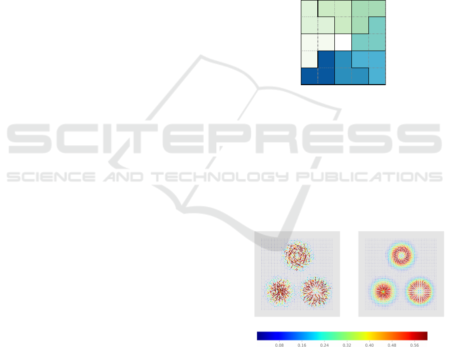
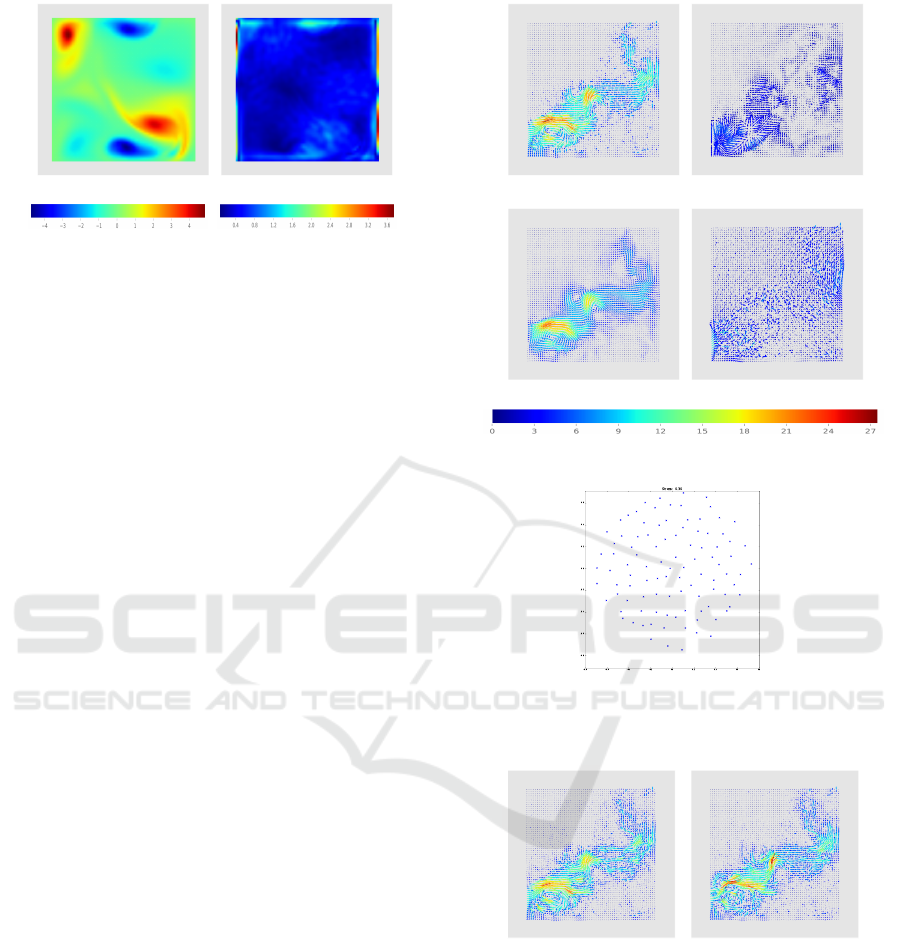
(a) Vector Field (b) Rotational-free term

Figure 1: The HHD states that a vector ﬁeld (a) is com-

posed of a rotational-free (b), a divergence-free (c), and a

harmonic component (d). The color bar represents the vec-

tor magnitudes.

where ∆ is the the Laplacian operator.

An important fact is that the HHD is unique for

vector ﬁelds vanishing at inﬁnity on unbounded do-

mains (Pascucci et al., 2014). However, to obtain

an unique solution for closed domains, some bound-

ary conditions should be established. The normal-

parallel (NP) boundary condition is the most com-

monly used, which requires the divergence-free and

the rotational-free components to be parallel and nor-

mal to the boundary, respectively:



∇ϕ ×n = 0

(∇ ·J)ψ ·n = 0

, (5)

where n represents the outward normal to the bound-

ary. Another possible boundary condition is to impose

constant potentials on the boundary, which implies

the rotational-free component normal to the boundary

and the divergence-free tangent to it (Petronetto et al.,

2010). However, these two types of boundary condi-

tions may introduce artifacts that were not observed in

the original ﬁeld due to the imposed dependency be-

tween the vector ﬁeld components and the shape and

orientation of the boundary. To overcome this prob-

lem, Pascucci et al. (Pascucci et al., 2014) proposed

the Natural HHD (NHHD), which decomposes V by

separating the components by its inﬂuences, which

can be internal or external. Its formulation is written

as follows:

V = ∇ϕ

∗

+ (∇ ·J)ψ

∗

+ h

∗

where, ∇ϕ

∗

is the natural divergence and (∇ ·J)ψ

∗

Bootstrapping Vector Fields

is the natural rotational. They represent the compo-

nents inﬂuenced by the divergence and rotational of

V inside the domain. Moreover h

∗

is the natural har-

monic, which is inﬂuenced only by the exterior of the

domain.

In this work, we adopted the NHHD method to

obtain the rotational-free, divergence-free and har-

monic natural components of a given 2D vector ﬁeld

V. More details for how to obtain this decomposition

can be found in the original work of (Pascucci et al.,

2014).

5 PROPOSED METHOD

This section presents a new stochastic method to gen-

erate 2D vector ﬁeld realizations from a given train-

ing data, i.e. a gridded 2D vector ﬁeld. This ap-

proach is based on the Bootstrap technique and uses

the Helmholtz-Hodge Decomposition to consistently

generate stochastic realizations of vector ﬁelds.

Consider a discrete sampling of a two-

dimensional domain on a Cartesian grid structure

m,n

= {x

i, j

∈ R

: 1 ≤ i ≤ m, 1 ≤ j ≤ n}. Also,

suppose that a discrete 2D vector ﬁeld V is given,

i.e., to each spatial point in S

m,n

there is a 2D vector

associated. This 2D vector ﬁeld V is the training

data.

The main goal of this method is to randomly gen-

erate vector ﬁelds that have similar characteristics of

the training one, i.e., that are structural perturbations

of the original vector ﬁeld.

Overview. The ﬁrst step in our method is to compute

the NHHD of the training data V. So, at each point

i, j

∈ S

m,n

we have the following equality:

∗

i, j

) = ∇ϕ

∗

i, j

)+(∇ ·J)ψ

∗

i, j

)+h

∗

i, j

). (6)

With the NHHD components of the given train-

ing data V in hand, we stochastically generate other

R 2D vector ﬁelds based on V. To obtain each real-

ization, we ﬁrstly perturb the divergence-free ϕ

∗

and

rotational-free ψ

∗

scalar potentials around b points

i, j

∈ S

m,n

using a Bootstrap-like technique. From

these perturbed scalar potentials, we then compute

the corresponding rotational-free and divergent-free

terms from their partial derivatives. We add these two

terms to the original harmonic term h

∗

in order to ﬁ-

nally create a vector ﬁeld realization.

The number b of blocks in which to perform the

Bootstrap is deﬁned through a Poisson Distribution

(Wasserman, 2004) with rate λ. This rate represents

the mean number of blocks that are going to be per-

turbed. The greater the λ the higher the variability

induced in the samples.

Given that we are dealing with vector ﬁelds, we

adopted an strategy to preserve their structure during

the resampling step. Such strategy is based on a ker-

nel proposed by (Fu et al., 2012) and depicted in Fig-

ure 2. This kernel explores the directional coherence

of the contours that pass through the central pixel.

As can be seen, the kernel divides a n ×n block in

8 subgroups. When performing the Bootstrap-based

technique, each of these regions is resampled with

replacement separately to obtain a Bootstrap sample

around the central pixel. The size of the kernel pre-

sented in Figure 2 is 5 ×5. The bigger the mask, the

higher the variation of the Bootstrap samples in rela-

tion to the input sample.

Figure 2: A kernel that divides a n ×n block of the domain

into 8 subgroups in order to preserve the vector ﬁeld orien-

tation after resampling with replacement the pixels in each

subgroup separately.

Once again, taking as a realization the vector ﬁeld

depicted in Figure 1, one can perceive, through Fig-

ure 3, that the adopted kernel is capable of preserving

the orientation of the vector ﬁeld used as input for

the Bootstrap method. More than that, in regions in

which the potentials are practically constant, no noise

is added to the vector samples.

(a) Example of a single sample (b) Mean of 100 samples

Figure 3: Example of vector ﬁelds obtained using a kernel

divided in regions to preserve the vector ﬁeld orientation.

The color scale matches the one presented in Figure 1 for

comparison purposes.

With this knowledge, we can now specify that, in

this work, λ is deﬁned as a percentage of the training

data size divided by the kernel size.

At last, a smoothing step is performed through a

Gaussian Filter (Gonzalez and Woods, 2006), which

GRAPP 2019 - 14th International Conference on Computer Graphics Theory and Applications

standard deviation (σ) can be parameterized, for both

x and y dimensions.

The Algorithm. We implemented the proposed

method according to the pseudocode described in Al-

gorithm 1. This pseudocode generates a stochastic

realization R

∗

based on the NHHD components of a

training data V.

The method has as input the following list of vari-

ables:

• the scalar potentials ϕ

∗

, ψ

∗

and the vector ﬁeld h

∗

obtained by the NHHD of the training data V;

• the kernel K of size l ×l used to perform the re-

sampling with replacement on the potentials;

• the number b of blocks in which we will perform

the Bootstrap.

Algorithm 1: Generation of a realization R

∗

based on the

NHHD components of a training 2D vector ﬁeld V.

input : ϕ

∗

, ψ

∗

, h

∗

, K, b

output: R

∗

, a vector ﬁeld realization

1 ϕ

∗

boot

← ϕ

∗

;

2 φ

∗

boot

← φ

∗

;

3 x ← randInt(1, m, b);

4 y ← randInt(1, n, b);

5 for k ← 1 to b do

6 i ← x[b] ;

7 j ← y[b] ;

8 boot indices ← local bootstrap(K);

9 ϕ

∗

boot

(i, j) ←

Fϕ(boot indices);

10 ψ

∗

boot

(i, j) ←

Fψ(boot indices);

11 end

12 ϕ

∗

boot

← smooth(ϕ

∗

boot

);

13 ψ

∗

boot

← smooth(ψ

∗

boot

);

14 ∇ϕ

∗

← divergent(ϕ

∗

boot

);

15 ∇ ×ψ

∗

← curl(ψ

∗

boot

);

16 R

∗

i, j

) ← ∇ϕ

∗

i, j

) + ∇ ×ψ

∗

i, j

) + h

∗

;

The input b deﬁnes the number of indexes that

will be generated through an Uniform Distribution

(Wasserman, 2004) (lines 3 and 4). These indexes

represent central positions of regions in the scalar po-

tentials of V that are going to be perturbed using a

Bootstrap-like approach.

Then, for each one of the b indexes pairs, say x

i, j

we perform a local bootstrap (line 8) centered on x

i, j

based on the input kernel K, which results in a new

organization of the l ×l region around x

i, j

. In other

words, the region around x

i, j

will be perturbed and

new values will be assigned to ?

∗

boot

(i, j).

In the following, we perform a smoothing step on

∗

boot

, i.e., we obtain a smoothed version of

. The

smoothing step is required because a small change in

the potentials can lead to a signiﬁcant change in the

vector ﬁeld, once this is obtained deriving these po-

tentials. In this work, we used σ equal to 2 pixels in

the smoothing step.

After these steps, we can now derive the new

scalar potentials to obtain new realizations for the

divergence-free (line 14) and rotational-free (line 15)

components of V. Finally, a new vector ﬁeld realiza-

tion is obtained summing these components with the

original harmonic component of V (line 16), follow-

ing Equation 2.

Repeating this procedure R times, we will then

have a set of R realizations of vector ﬁelds obtained

through the original NHHD components of V.

6 RESULTS AND DISCUSSION

To verify the results that the proposed method can

achieve, we make use of a 2D vector ﬁeld ensem-

ble comprehended by seven multi-method wind fore-

cast realizations E , provided by the Brazilian Instituto

Nacional de Pesquisas Espaciais (INPE). Each real-

ization in E represent a possible wind forecast for a

region delimited by 35

◦

S and 83

◦

W as the mini-

mum latitude and longitude coordinates (DMS), re-

spectively, and by 6

◦

N and 25

◦

W as the max-

imum latitude and longitude coordinates, in that or-

der. The data is deﬁned over a Cartesian grid structure

with dimension of 144 ×106.

As a ﬁrst step, we apply the NHHD on each

realization R in E to derive its divergence-free,

rotational-free and harmonic components. Through

this decomposition, we obtain the potentials of the

rotational-free and divergence-free components. With

those potentials in hand, we can then derive the

rotational-free, divergence-free and harmonic compo-

nents as stated in Equation 2. For each realization R

in E , we apply Algorithm 1 to obtain 100 other new

realizations.

Similarity Measure and MDS Projection. To pro-

vide a way of visually encode the similarity between

the vector ﬁelds, we make use of the MDS (Kruskal,

1964) technique for dimensionality reduction to visu-

alize high-dimensional data in a 2-dimensional space.

The MDS method aims to provide insight in the un-

derlying structure and relations between patterns by

providing a geometrical representation of their sim-

ilarities (Honarkhah and Caers, 2010). Mathemat-

ically speaking, MDS translates a dissimilarity ma-

Bootstrapping Vector Fields

trix into a conﬁguration of points in a n-D Euclidean

space.

For two vector ﬁelds A and B, we adopted the fol-

lowing similarity measure, known as the Cosine Sim-

ilarity:

similarity

A,B

= cos θ =

A ·B

kAk·kBk

(7)

Such a measure states how related two vector

ﬁelds are given their angles. For similar vectors the

similarity coefﬁcient will be close to 1, for opposite

vectors, such coefﬁcient will be close to −1. For un-

related vectors, on the other hand, this coefﬁcient will

be around 0.

To take into account both the magnitude and ori-

entation of the vector ﬁelds A and B in the cosine sim-

ilarity computation, we perform the following trans-

formation.

Firstly, for a vector V of dimensions m×n, we un-

roll it from a 2-dimensional vector to a 1-dimensional

vector. Then, we generate a new vector V

∗

= (v

∗

)

based on V such as:

∗

= atan2(v

)

∗

= kVk

∗

= (v

)

For an ensemble E , after this step, we have a new

set E

∗

in hand. All vectors in E

∗

are normalized as

follows:

∗

π/2

∗

max(v

∗

∈ E

∗

)

After this transformation, we apply the similarity

measure for each pair of realizations in E

∗

Figure 4 presents the MDS for the wind fore-

cast ensemble and its mean vector, after applying the

transformation described before.

Figure 4: MDS visualization for the original ensemble E .

Colors represent each realization in E . The black square

represent the mean vector of E .

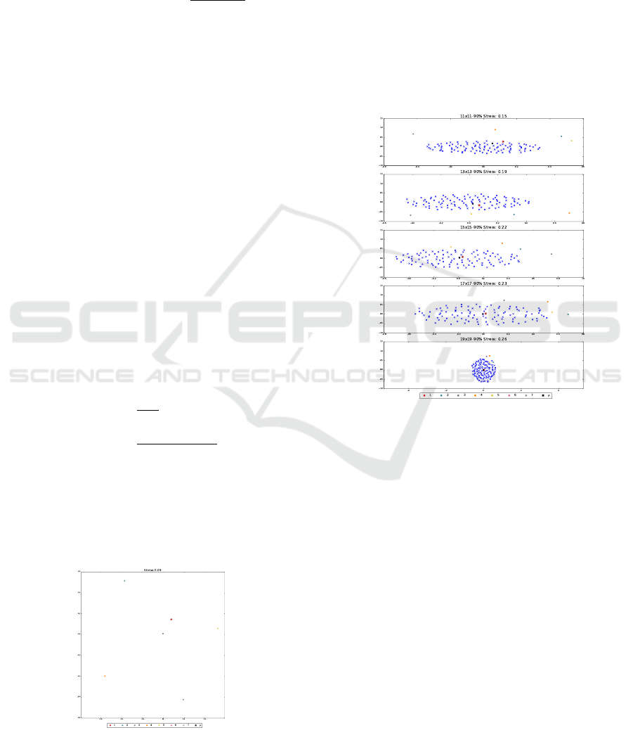
Coverage Test. It is relevant to verify whether we

can generate a set of realizations that covers the given

ensemble set or not. This might state if, from a sin-

gle realization, it is possible to obtain certain scenar-

ios that could be derived through another simulation

process (possible more costly). To do this, we ﬁrst

tried different values for the λ parameter given differ-

ent bootstrap kernel sizes to generate 100 new sam-

ples from the mean vector ﬁeld µ. They ranged from

30% to 90% and from 5 ×5 to 17 ×17, respectively.

We achieved the best coverage using a λ value of

90% and a kernel size of 19 ×19, as can be seen in

Figure 5.

Figure 5: MDS visualization between E and a new ensam-

ble generated through the mean of E , represented as a black

square.

Given that, Figure 6 present the MDS for each

vector ﬁeld in the original set E and a new set of re-

alizations derived from it using a kernel size and λ

as speciﬁed before. Markers of same color belongs

to the same set, i.e, were generated based on a com-

mon realization. Circle markers represent each re-

alization of the set E . Cross markers represent new

realizations, and square markers show both the clos-

est and farthest simulation given a base realization –

Table 4 depict these simulations for each realization

in E . Through this image, we can see that, for each

realization s ∈ (1,··· ,7), the resulting set of realiza-

tions present some variability in relation to the origi-

nal vector ﬁeld used as base for the stochastic simula-

tion method.

Putting all these simulations together, we have the

result presented in Figure 7. From this image, we can

notice that the original set E is completely surrounded

by the new realizations.

GRAPP 2019 - 14th International Conference on Computer Graphics Theory and Applications

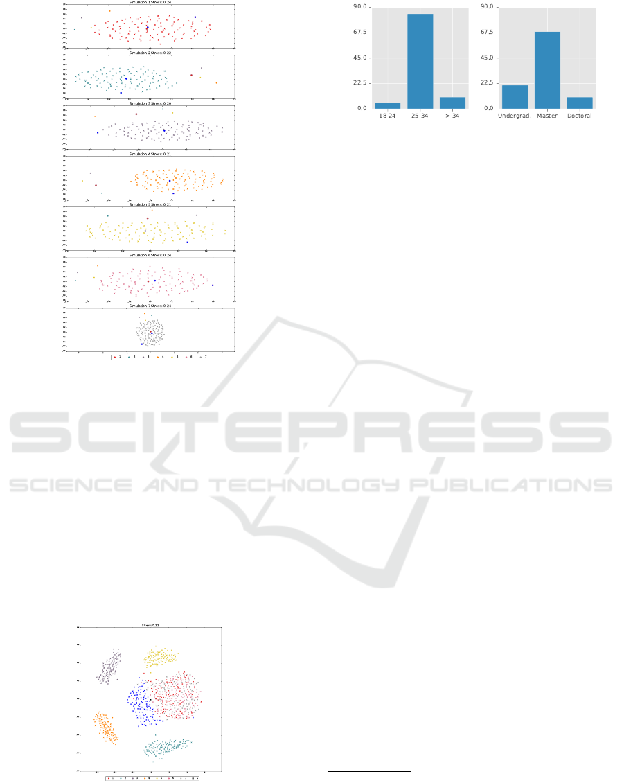
Figure 6: MDS visualization between each set of new real-

izations and the original ensemble E . Colors represent each

realization of the set E . Circular markers represent each re-

alization in E . Cross markers represent, for each V in E , the

new realizations derived from V, both presenting the same

color.

Evaluation. Willing to evaluate the quality of the

results achieved with the proposed method, we con-

ducted an informal study with 19 people with a var-

ied age range as well as educational level (Figure 8).

Here, we deﬁne quality as the capacity of a generated

realization be as realistic as the input data set (1) and

unique in comparison with its members (2).

To evaluate (1) we displayed 4 vector ﬁelds (2 of

Figure 7: MDS visualization between each new realization

and the original ensemble E . Colors represent each realiza-

tion of the set E . Circular markers represent each realiza-

tion in E. Cross markers represent new realizations derived

from the original one (presented with a circular marker of

the same color).

(a) Age (b) Level of Education

Figure 8: Summary of the 19 participants of our informal

study.

them from the wind forecast data set – members 1 and

– and the other 2 generated through the proposed

method – realizations 4f and 7c) and asked the par-

ticipants to classify them as training or stochastically

generated or choose the option I don’t know. Most

of the participants got the right answer, however, for

a close call. For instance, training data 5 was cor-

rectly classiﬁed by 57.9% of the participants, while

21.1% classiﬁed it as stochastically generated and the

remaining couldn’t tell the difference. The same re-

sult was observed for the stochastically generated vec-

tor ﬁeld 7c. On average, 60.55% of the participants

chose the correct answer, 21% chose the wrong an-

swer and 18.45% didn’t know how to classify it.

For the evaluation of (2) we presented two sets of

vector ﬁelds. The ﬁrst one contained 3 members of

the wind forecast data set (members 1, 2 and 3). The

second one was composed by 3 vector ﬁelds (realiza-

tions 1c, 2c and 3c) generated using the ﬁrst set mem-

bers. We then asked the participants to indicate, for

each member of the second set, which vector ﬁeld in

the ﬁrst one was used to generate it, or the option I

don’t know. For all vector ﬁelds in the second set, the

majority of the participants did not identify the cor-

rect training vector ﬁeld. The percentage that did it

was 10.5%, 21.1% and 10.5%, for each vector ﬁeld

in the second set. For the ﬁrst vector ﬁeld in this

set, 1c, 31.1% of the participants couldn’t chose the

most similar vector ﬁeld from the original data set.

For the second and third vector ﬁelds, this percentage

was 21.1%. Realization 3c was characterized as al-

most similar to two different vector ﬁelds (31.6% for

3 and 36.8% for 1), being considered more similar to

a vector ﬁeld different from its training one.

These results show that, despite being possible to

identify the tested vector ﬁelds as training or stochas-

For all data used in this test and here presented, read

Table 4 as:

1. member x: x-th vector ﬁeld in column Realization;

2. xc: x-th vector ﬁeld in column Closest Simulation;

3. xf: x-th vector ﬁeld in column Farthest Simulation.

Bootstrapping Vector Fields

tically generated, our method was capable to generate

realizations that mimics the physical simulation.

7 APPLICATIONS

As mentioned before, the presented approach may be

useful in a varied range of applications. In this sec-

tion, we present a quantiﬁcation approach to the algo-

rithm uncertainty related to different scenarios of the

curl and divergence discrete differential operators.

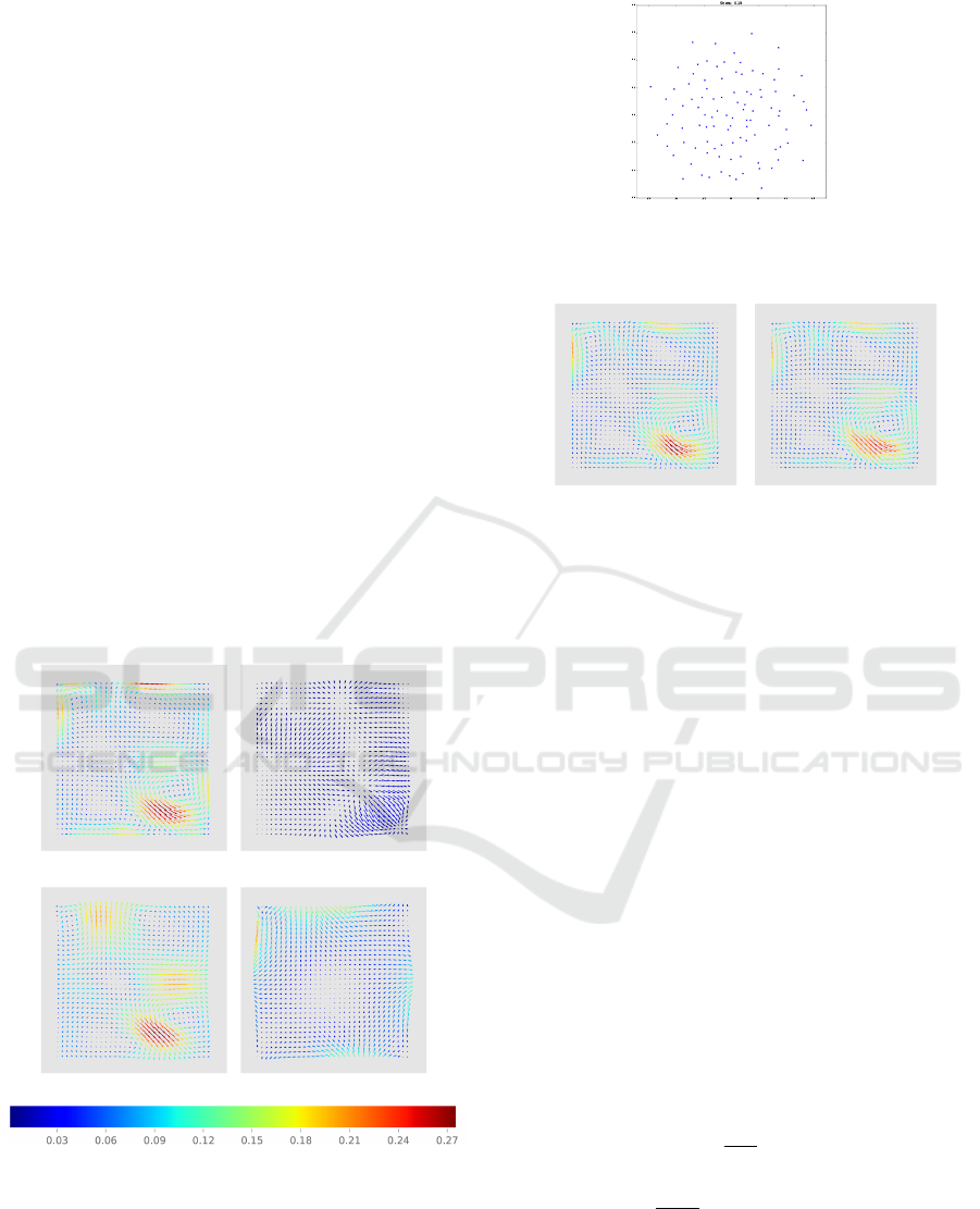
Navier-Stokes. Consider the vector ﬁeld presented

in Figure 9. This ﬁeld is deﬁned over a grid of

64×64, with its minimum and maximum as 0.007812

and 0.992188, respectively, in the x and y directions.

This ﬁeld is the result of a Navier-Stokes simulation

(Chorin, 1968), which aims to describe the motion

of viscous ﬂuid ﬂows. Such kind of simulation can

be used to model a varied set of physics phenomena,

ranging from waves simulation (Abadiea et al., 2010)

to image and video inpainting (Bertalmio et al., 2001).

As can be seen, the divergence-free component de-

ﬁnes such ﬁeld (we may consider the rotational-free

and harmonic components as noise).

(a) Vector Field (b) Rotational-free

Figure 9: Navier-Stokes simulation and its NHHD compo-

nents.

After generating 100 new realizations through the

procedure presented in Algorithm 1, using a kernel

of 5 ×5, we have a set of realizations E . Figure 10

shows the MDS for this set. As can be seen, the orig-

inal sample is surrounded by the new ones.

Figure 10: MDS visualization between each new realization

and the original realization. Samples generated using a 5×5

kernel.

(a) Closest Simulation (b) Farthest Simulation

Figure 11: Closest and farthest simulation of the Navier-

Stokes vector ﬁeld.

Figure 11 shows the closest and farthest simula-

tion derived from the original vector ﬁeld. They are

represented using the same magnitude scale as the

original ﬁeld (Figure 9).

With this set in hand, it is now possible to quan-

tify the uncertainty related to the curl operator, which

is obtained using partial derivatives. In other words,

we can measure the uncertainty related to the kernel

used to obtain such attribute. To do so, for each new

realization R ∈E , we obtain the curl of R. We do the

same for the original sample V. To derive the uncer-

tainty of the curl operator, we then compute its mean

squared error (RMSE).

In statistics, the mean squared error, MSE, of an

estimator is a way to measure the difference between

values implied by an estimator and the true values of

its target parameter (Wackerly et al., 2008).

For instance, being

T the curl of V and T

∗

, i =

1,.. .,100 the curl of each one of the generated sam-

ples, the MSE of the predictor

T is deﬁned as:

MSE(

T) =

100

∑

i=1

(

T −T

∗

)

(8)

The RMSE is given as the square root of the MSE,

i.e., RMSE =

√

MSE.

Figure 12 presents the RMSE of the curl given the

generated realizations.

GRAPP 2019 - 14th International Conference on Computer Graphics Theory and Applications

(a) Curl of V (b) RMSE of the curl

Figure 12: Curl of V (a) and RMSE of the curl operator (b)

between the set E and the realization V.

Particle-Image Velocimetry. Often, PIV applica-

tions aims to study the behavior of turbulent ﬂows, an-

alyzing the stability of features such as vortices. Be-

sides providing means to perform this kind of study

through the generation of different realizations, we

can go further with the new samples generated using

the proposed technique.

The following PIV simulation is deﬁned over a

grid of 124 ×126. Its horizontal dimension ranges

from 0.3824 to 47.4176. On the other hand, its verti-

cal dimension ranges from 0.3824 to 48.1824. Figure

13 shows this vector ﬁeld, as well as its NHHD com-

ponents. This image corresponds to a velocity ﬁeld of

a gas ﬂow that is continuously injected horizontally

on the bottom left corner and that ﬂows on the domain

from left to right until it meets a wall (image’s right

edge). It is possible to observe that the divergence-

free component seems to have a high magnitude and

basically dominate the ﬂow behavior; we can also no-

tice that the rotational-free component present some

features that characterize it.

Figure 14 presents the MDS between the new re-

alizations (generated using a kernel of size 19 ×19)

and the original one. Once again, the training data is

surrounded by the generated realizations.

Figure 15 shows the closest and farthest simula-

tion derived from the original vector ﬁeld. They are

represented using the same magnitude scale as their

original ﬁeld (Figure 13).

From Figure 16, we can see that, for the curl oper-

ator, the RMSE is higher on regions with high magni-

tude. In such areas, the scalar ﬁeld also present high

values. So, a small change in these regions are capa-

ble of generating a great change in the vector ﬁeld.The

same behavior happens with the divergence operator,

i.e., we have a higher uncertainty in areas where the

magnitude of the vector ﬁeld is also higher.

(a) Vector Field (b) Rotational-free

Figure 13: PIV simulation and its NHHD components.

Figure 14: MDS visualization between each new realization

and the original realization. Samples generated using a 19×

19 kernel.

(a) Closest Simulation (b) Farthest Simulation

Figure 15: Closest and farthest simulation of the Navier-

Stokes vector ﬁeld.

8 PERFORMANCE

Here we present the performance of the proposed

technique. Tests were performed using a machine

running ubuntu 16.04 LTS with the conﬁguration pre-

sented in Table 1.

For each data set presented in this paper, we mea-

sured the time necessary to compute the NHHD and

to generate new realizations (as the mean of the time

Bootstrapping Vector Fields

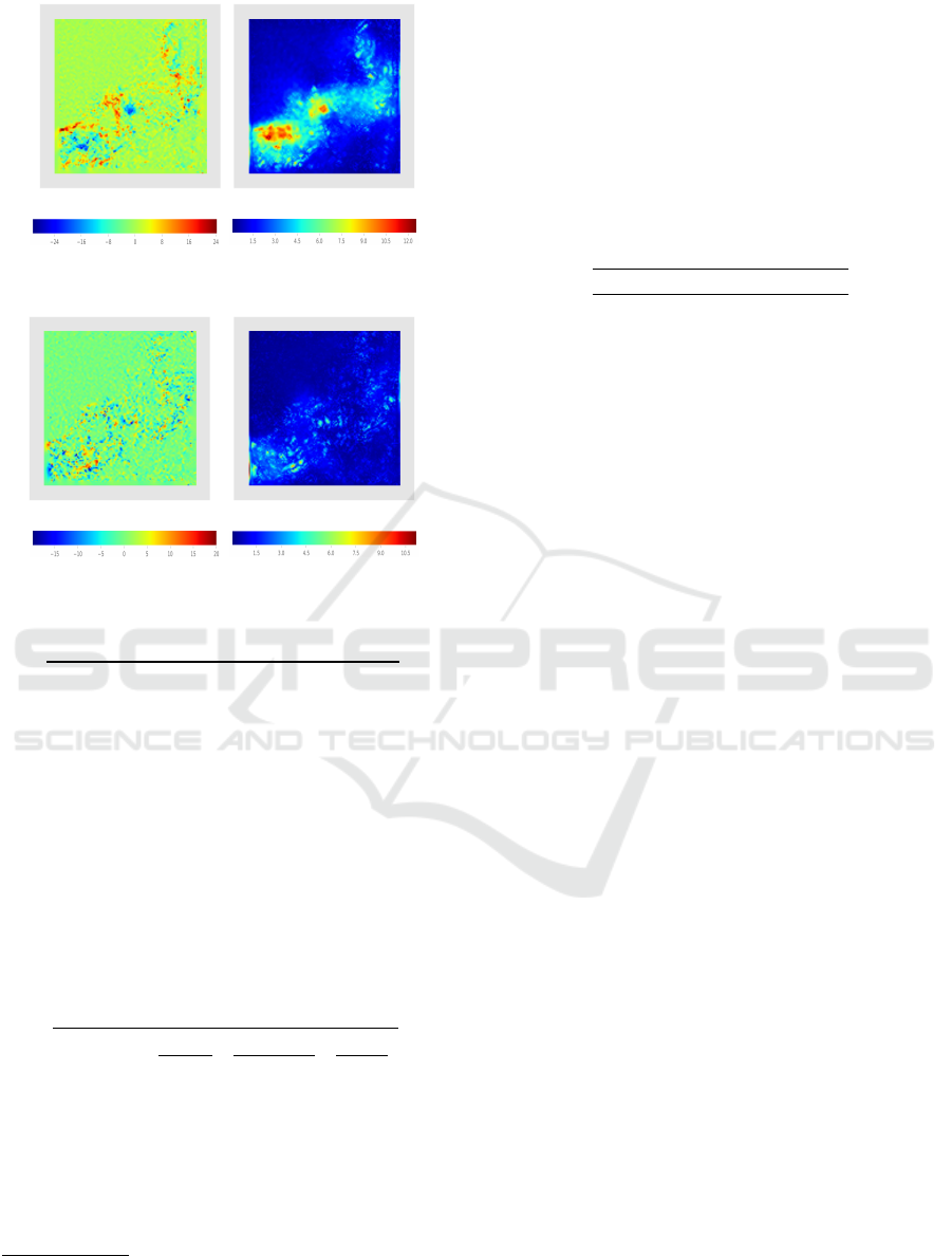
(a) Curl of V (b) RMSE of the curl

Figure 16: Curl of V (a) and RMSE of the curl operator (b)

between the set E and the realization V.

(a) Divergence of V (b) RMSE of the divergence

Figure 17: Divergence of V (a) and RMSE of the divergence

operator (b) between the set E and the realization V.

Table 1: Machine conﬁguration.

Memory 62.8 GiB

Processor Intel



Core

i7-5820K CPU @ 3.30 GHz ×12

Graphics GeForce GTX 960/PCle/SSE2

OS Type 64 bit

Disk 55 GB

spent to generate a set with 100 new samples). Those

can be seen in Table 2. It is important to notice that

all methods here presented, as well as the time mea-

surement, were coded in Python 2.7, using the Numpy

numerical library and the SciPy library of scientiﬁc

tools.

Table 2: Performance of the proposed method per sample,

in seconds. Tested using λ equal to 90% for all scenarios

and a kernel of 15 ×15.

Forecast

Navier-Stokes

PIV

NHHD 1025.775 86.497 1200.545

Samples Gen. 0.584 0.209 0.992

As can be seen, the NHHD is the most time con-

suming step. For more details on the performance of

the NHHD, see (Pascucci et al., 2014).

We also tested the effect of different kernel sizes

on the samples generation step. This is shown in Ta-

19 ×19 kernel.

5 ×5 kernel.

19 ×19 kernel.

ble 3. As we can observe, the size of the kernel didn’t

cause a signiﬁcant change in the algorithm perfor-

mance. It is also interesting to note that, the bigger

the size of the kernel the lesser the time consump-

tion. This means that the bootstrap step performance

is mostly affected by the number of blocks chosen,

instead of the size of the chosen kernel.

Table 3: Performance of the sample generation step for dif-

ferent kernel sizes. Tested with the wind forecast ensemble

mean and λ equal to 90%.

11 ×11 13 ×13 15 ×15 17 ×17

0.613 0.612 0.580 0.577

9 CONCLUSION

This paper proposed a technique to stochastic simu-

late vector ﬁelds given a single realization. Thanks

to the Helmholtz-Hodge Decomposition method we

could develop a method that provides a good level

of realistic scenarios. To the best of our knowledge,

this is the ﬁrst approach that uses the Helmholtz-

Hodge Decomposition to stochastic generate vector

ﬁelds given a training data. Results were evaluated us-

ing a set of multi-method wind forecast realizations,

as well as simulations from Navier-Stokes and PIV.

For each data, 100 new scenarios were generated us-

ing the presented method. We applied the MDS tech-

nique to proper visualize the results; we could ob-

serve that the simulated scenarios were able to pro-

vide a great variability and that they mimic the train-

ing data. The applicability of this approach ranges

from uncertainty quantiﬁcation to data assimilation

(Kalnay, 2003). Further studies includes expanding

this method for 3-dimensional vector ﬁelds, as well

as exploring other techniques for random vector ﬁeld

synthesis.

ACKNOWLEDGEMENTS

We would like to thank CAPES and CNPq for the

ﬁnancial support of this research. Additionally, we

would like to thank INPE and Haroldo Fraga de Cam-

pos Velho for the wind forecast data models used in

this work.

REFERENCES

Abadiea, S., Morichona, D., Grillib, S., and Glockner, S.

(2010). Numerical simulation of waves generated by

landslides using a multiple-ﬂuid NavierStokes model.

Coastal Engineering, 57(9):779–794.

GRAPP 2019 - 14th International Conference on Computer Graphics Theory and Applications

Anderson, J. D. and Wendt, J. (1995). Computational ﬂuid

dynamics, volume 206. Springer.

Beccali, M., Cellura, M., and Mistretta, M. (2003).

Decision-making in energy planning. application of

the electre method at regional level for the diffusion

of renewable energy technology. Renewable Energy,

28(13):2063–2087.

Bertalmio, M., Bertozzi, A. L., and Sapiro, G. (2001).

Navier-stokes, ﬂuid dynamics, and image and video

inpainting. In Proceedings of the 2001 IEEE Com-

puter Society Conference, pages 355–362. IEEE.

Bhatia, H., Norgard, G., Pascucci, V., and Bremer, P.

(2013). The Helmholtz-Hodge Decomposition - A

Survey. IEEE Transactions on Visualization and Com-

puter Graphics, 19(8):1386–1404.

Cho, K., Meer, P., and Cabrera, J. (1997). Perfor-

mance assessment through bootstrap. IEEE Transac-

tions on Pattern Analysis and Machine Intelligence,

19(11):1185–1198.

Chorin, A. J. (1968). Numerical solution of the Navier-

Stokes equations. Mathematics of Computation,

22:745–762.

Chorin, A. J. and Marsden, J. E. (1993). A mathematical in-

troduction to ﬂuid mechanics. Texts in Applied Math-

ematics. Springer-Verlag, 3rd edition.

Efron, B. (1979). Bootstrap Methods: Another Look at the

Jackknife. Annals of Statistics, 7:1–26.

Efros, A. A. and Freeman, W. T. (2001). Image quilting

for texture synthesis and transfer. In Proceedings of

the 28th annual conference on Computer graphics and

interactive techniques, pages 341–346. ACM.

Fu, X., You, H., and Fu, K. (2012). A Statistical Approach

to Detect Edges in SAR Images Based on Square Suc-

cessive Difference of Averages. IEEE Geoscience And

Remote Sensing Letters, 9(6):1094–1098.

Gao, H., Mandal, M. K., Guo, G., and Wan, J. (2010). Sin-

gular point detection using Discrete Hodge Helmholtz

Decomposition in ﬁngerprint images. In ICASSP’10,

pages 1094–1097. IEEE.

Gonzalez, R. C. and Woods, R. E. (2006). Digital Image

Processing. Prentice-Hall, Inc.

Guo, Q., Mandal, M. K., Liu, G., and Kavanagh,

K. M. (2006). Cardiac video analysis using Hodge-

Helmholtz ﬁeld decomposition. Computers in Biology

and Medicine, 36(1):1–20.

Honarkhah, M. and Caers, J. (2010). Stochastic Simulation

of Patterns Using Distance-Based Pattern Modeling.

Mathematical Geosciences, 42(5):487–517.

Kalnay, E. (2003). Atmospheric modeling, data assimila-

tion and predictability. Cambridge university press.

Kruskal, J. B. (1964). Multidimensional scaling by optimiz-

ing goodness of ﬁt to a nonmetric hypothesis. IEEE

Transactions on Visualization and Computer Graph-

ics, 29(1):1–27.

Lall, U., Devineni, N., and Kaheil, Y. (2016). An empiri-

cal, nonparametric simulator for multivariate random

variables with differing marginal densities and nonlin-

ear dependence with hydroclimatic applications. Risk

Analysis, 36(1):57–73.

Lantu

ejoul, C. (2013). Geostatistical simulation: models

and algorithms. Springer Science & Business Media.

Liew, K. J., Ramli, A., and Majid, A. A. (2016). Searching

for the optimum value of the smoothing parameter for

a radial basis function surface with feature area by us-

ing the bootstrap method. Computational and Applied

Mathematics, pages 1–16.

Luo, C., Safa, I., and Wang, Y. (2012). Feature-aware

streamline generation of planar vector ﬁelds via topo-

logical methods. Computers & Graphics, 36(6):754–

766.

Mariethoz, G. and Caers, J. (2014). Multiple-point geo-

statistics: stochastic modeling with training images.

John Wiley & Sons.

Mariethoz, G. and Lefebvre, S. (2014). Bridges between

multiple-point geostatistics and texture synthesis: Re-

view and guidelines for future research. Computers &

Geosciences, 66:66–80.

Oliver, M. and Webster, R. (2014). A tutorial guide to geo-

statistics: Computing and modelling variograms and

kriging. Catena, 113:56–69.

Palit, B. (2005). Application of the Hodge Helmholtz De-

composition to Video and Image Processing. Master’s

thesis, University of Alberta.

Pascucci, V., Bremer, P.-T., and Bhatia, H. (2014). The

Natural Helmholtz-Hodge Decomposition For Open-

Boundary Flow Analysis. IEEE Transactions on Vi-

sualization and Computer Graphics, 99(PrePrints):1–

11.

Petronetto, F., Paiva, A., Lage, M., Tavares, G., Lopes, H.,

and Lewiner, T. (2010). Meshless Helmholtz-Hodge

Decomposition. IEEE Transactions on Visualization

and Computer Graphics, 16(2):338–349.

Polthier, K. and Preuß, E. (2003). Identifying Vector Field

Singularities Using a Discrete Hodge Decomposition.

In Visualization and Mathematics III, pages 113–134.

Springer Berlin Heidelberg.

Popescu, R., Deodatis, G., and Prevost, J. H. (1998). Simu-

lation of homogeneous nongaussian stochastic vector

ﬁelds. Probabilistic Engineering Mechanics, 13(1):1–

13.

Ribeiro, P. C., de Campos Velho, H. F., and Lopes, H.

(2016). Helmholtz-hodge decomposition and the anal-

ysis of 2d vector ﬁeld ensembles. Computers &

Graphics, 55:80–96.

Tong, Y., Lombeyda, S., Hirani, A. N., and Desbrun, M.

(2003). Discrete Multiscale Vector Field Decomposi-

tion. In ACM SIGGRAPH 2003 Papers, pages 445–

452. ACM.

Wackerly, D. D., Mendenhall, W., and Scheaffer, R. L.

(2008). Mathematical Statistics with Applications.

Thomson.

Wang, H. and Deng, J. (2014). Feature extraction of com-

plex ocean ﬂow ﬁeld using the helmholtz-hodge de-

composition. In 2013 IEEE International Confer-

ence on Multimedia and Expo Workshops, pages 1–6.

IEEE.

Wang, Z., Wang, X., and Ji, Q. (2014). Learning with hid-

den information. In ICPR, pages 238–243.

Wasserman, L. (2004). All of Statistics: A Concise Course

in Statistical Inference. Springer.

Xiu, D. (2009). Fast numerical methods for stochastic com-

putations: a review. Communications in computa-

tional physics, 5(2-4):242–272.

Bootstrapping Vector Fields

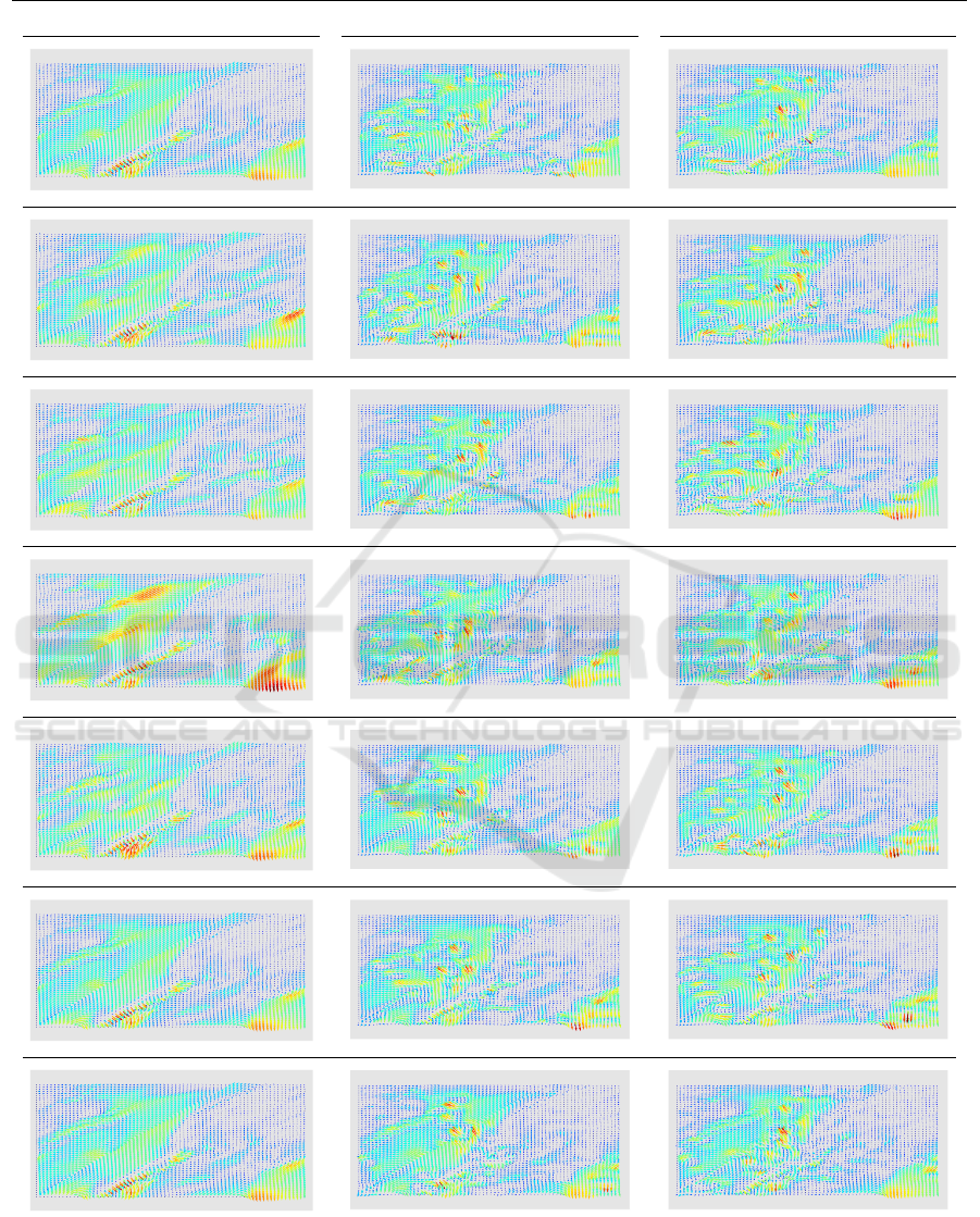
Table 4: Original realization and its closest and farthest simulation.

Realization Closest Simulation Farthest Simulation

GRAPP 2019 - 14th International Conference on Computer Graphics Theory and Applications