
Determining Equilibrium Staffing Flows in the Canadian Department
of National Defence Public Servant Workforce
Etienne Vincent and Stephen Okazawa
Director General Military Personnel Research and Analysis, Department of National Defence,
101 Colonel By Dr, Ottawa, Canada
Keywords: Personnel Modelling, Workforce Analytics, Staffing Requirements, Human Resources Planning, Attrition
Rate.
Abstract: In large workforces, such as the Public Servant workforce of the Canadian Department of National Defence,
many staffing actions (hires, departures, promotions, transfers) are actioned each year. Estimating the number
of such actions that will take place in the department’s various units is relevant to the assignment of Human
Resource support capacity. The rates at which staffing actions are required is also indicative of the health of
workforce occupational segments. This paper presents a method for estimating the number of staffing actions
that will be required to maintain a workforce to a state of equilibrium. It also shows how that method was
practically implemented in support of Strategic Human Resource Planning for Canada’s Department of
National Defence civilian workforce.
1 BACKGROUND
The Department of National Defence (DND) and
Canadian Armed Forces make up the largest
Canadian federal government department. In
addition to uniformed Regular and Reserve Force
members, approximately 25,000 Public Servants are
employed in the department.
The model described in this paper was developed
at the request of DND’s Assistant Deputy Minister
(Human Resources – Civilian), who has a need to
monitor and predict the number of staffing actions
taking place within the department’s Public Servant
workforce. Staffing actions are the movements of
personnel in and out of departmental positions. As
such, they include hiring, departures, promotions and
transfers.
Monitoring and predicting staffing actions is of
interest for two reasons. First, it informs the
assignment of Human Resources support capacity to
where it is needed (having the right number of Human
Resources staff to process staffing actions in each
unit). Secondly, the volume of staffing actions
informs occupational health assessments across the
department (e.g. high attrition, high transfer, or low
promotion rates could be indicators of unhealthy
workforce dynamics).
Workforce dynamics have often been investigated
through simulation, such as Markov modelling
(Mitropoulos, 1983; Georgiou, 1999), or Discrete
Event Simulation (Okazawa, 2013; Zegers and
Isbrandt, 2010). Instead, we take the approach of
explicitly solving for staffing flows in a personnel
system under an assumption of equilibrium. This is
similar to (Bartholomew, 1969), but extended to
consider both push and pull staffing actions. It is also
similar to (Doumic et al, 2016), which represents
staffing flows as differential equations, but focuses on
workforce age profiles as the determinant of flows,
rather than the occupation and level studied in this
paper. In the case of a rigid military personnel
system, additional control over recruitment (always
into the lowest rank), promotion policy, terms of
service, etc. allow for direct optimization, such as in
(Marquez and Nelson, 1996 or Filinkov et al, 2011).
Explicit optimization is not as helpful in more fluid
Public Service workforces, so we take the approach
of describing the flows in the system, an endeavour
that Human Resource Planners find useful in its own
right. This paper describes the processes developed to
model and report the Public Servant staffing flows of
the DND.
Vincent, E. and Okazawa, S.
Determining Equilibrium Staffing Flows in the Canadian Department of National Defence Public Servant Workforce.
DOI: 10.5220/0007246802050212
In Proceedings of the 8th International Conference on Operations Research and Enterprise Systems (ICORES 2019), pages 205-212
ISBN: 978-989-758-352-0; ISSN: 2184-4372
Copyright
c
2023 by His Majesty the King in Right of Canada as represented by the Minister of National Defence and SCITEPRESS – Science and Technology Publications, Lda. Under
CC license (CC BY-NC-ND 4.0)
205
2 STAFFING ACTIONS
Canadian Public Servants are classified according to
the Occupational Group Structure, which is
composed of Groups, Classifications and Sub-groups.
For ease of presentation, we will refer to the various
sub-divisions of the structure as occupations. Each
occupation is then broken down into levels, which
correspond to successive salary ranges and seniority.
In examples, this paper refers to the Financial
Management Classification (denoted
FI
). It is broken
down into four levels,
FI01
being the junior level, and
FI04
the senior.
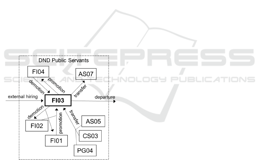
Public Servants hold positions at a set occupation
and level. Figure 1 depicts various staffing actions
that could result in an employee moving in or out of
the
FI03
occupation-level. The employee can be
promoted to
FI04
, or less commonly demoted to
FI02
or
FI01
, or could transfer to any other occupation (the
transfer to Administrative Services (
AS07
) is shown
as it is the most common destination for
FI03
employees). An
FI03
employee could also depart the
DND workforce completely, for retirement or another
reason. Figure 1 also shows the similar movements
into
FI03
(external hiring, promotion, demotion and
transfer).
Figure 1: Staffing actions for the FI03 occupation-level.
There is another type of staffing action that is not
depicted in Figure 1 and that can be important to
Human Resources Planning – lateral transfers (e.g.
transfers to a different
FI03
position elsewhere in the
DND). These can constitute a substantial portion of
overall staffing turnover, but lie outside the model
presented in this paper. If needed, lateral transfers
can easily be considered separately from the model
presented in this paper.
This paper aims to quantify the expected annual
flows in and out of occupation-levels. To do so, it
relies on historical data describing past flows. In
practice, we have access to annual workforce
snapshots and counts of staffing actions, tallied by
occupation and level.
3 THE DEPARTMENTAL
WORKFORCE
Let w=
,
,…,
be a workforce, where each
is the number of employees of a given occupation
and level (with the subscript denoting the occupation-
level pair). Our goal is to estimate the number and
type of staffing actions that should be expected each
year when the workforce is at equilibrium.
Each year, some employees depart w, change
level through promotion, and transfer between
occupations. Then, new employees are hired to fill
the gaps. This paper presents an approach to
estimating the number of such staffing actions that are
expected to occur in a workforce at equilibrium, from
historical data that are not necessarily from a system
at equilibrium.
Note that equilibrium is not necessarily the most
relevant state to be modelled from the perspective of
Human Resources Planning. It is explored in this
paper as the relevant base case, in the absence of more
definite Human Resources plans. Incorporating
planned growth or reductions into the model that is
developed below is trivial, if such plans exist. In any
case, when assessing the health of the occupation,
equilibrium flows a useful indicator of what would be
required to maintain the status quo.
4 ATTRITION
This section describes how to apply workforce
attrition rates. The process used to estimate attrition
rates from historical data will be described later. Let
be the historically observed annual attrition rate
among employees of occupation-level . Here,
attrition is defined as departing w altogether. If there
are
employees at a given occupation-level at the
beginning of the year, and assuming no hiring or
movements between occupation-levels, we expect
that
·
of them will have departed by year end,
and therefore, that
·(1−
) will remain.
However, attrition does not only apply to the
employees who are initially in the workforce.
Employees externally hired in the course of the year
ICORES 2019 - 8th International Conference on Operations Research and Enterprise Systems
206
are also subject to the attrition rate. If ℎ
employees
are hired at date (expressed a proportion of the year),
we expect that ℎ
∙
(
1−
)
of them will remain at
year end.
If we knew the precise dates on which new hires
will join the workforce, we would use this
information to determine the expected attrition
among hires. However, we do not generally know the
dates of future staffing actions – we likely only have
annual staffing targets. In order to apply attrition to
future hires, we need to make an assumption about
how they will be distributed in time. In the absence
of other information, we assume, as in (Okazawa,
2007; Fang and Bender, 2008), that they will be
uniformly spread. Thus, among the ℎ
hires at
occupation-level over a given year, we expect that
ℎ
(
1−
)
=ℎ
−
ln
(
1−
)
≡ℎ
∙
(1)
will remain at the end of the year (
is introduced for
ease of notation in follow-on equations). Attrition
among employees coming in or out of
through
promotion or transfer can be similarly handled.
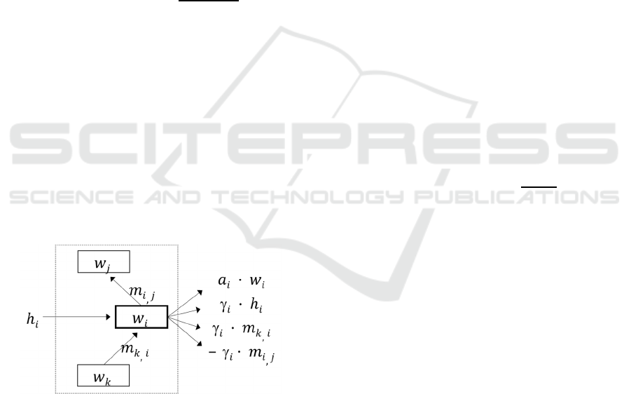
5 STAFFING FLOWS
We now turn our attention to the balance of annual
flows in and out of
. These are depicted in Figure
2.
Figure 2: Staffing flows in and out of
.
First are the flows that are internal to w – flows
between occupation-levels. Let
,
be the annual
movement of employees from
to
. Figure 2 only
shows one such flow into
, and one out, but such
flows in and out can potentially exist between
and
all of the other levels. The inflow into
from
outside w corresponds to external hiring, and is
denoted ℎ
.
Figure 2 also shows four types of attrition
(external outflows) which we will now describe in
turn. Basic attrition from
is obtained by applying
the relevant attrition rate as
·
. However, we
must also account for the effect of hiring and internal
movements on attrition. As described in Equation
(1),
∙ℎ
is the attrition among new hires. Similarly,
there can be attrition among employees that flow into
from other occupation-levels. If these flows are
assumed to occur uniformly throughout the annual
period, then the situation is as in Equation (1), and the
attrition from these inflows is
·
,
for each .
Finally, –
·
,
accounts for the reduction in
attrition out of
as a result of the
,
outflow. Note
that the last three attrition flows from Figure 2 simply
amount to applying the rate
to the net inflow.
Now, if the headcount
is to remain unchanged
from year to year, all of the annual flows in and out
of
must exactly balance out. Thus,
0=ℎ
+
,
−
,
−
−
ℎ
−
,
+
,
(2)
which simplifies to
0=ℎ
+
,
−
,
−
1−
∙
(3)
6 PUSH STAFFING FLOWS
In order to use Equation (3) to determine staffing
flows, further assumptions are necessary. We will
use the two types of internal flows described by
(Bartholomew et al, 1991) and that we believe
adequately describe most real world staffing
phenomena: push and pull flows.
Push flows are those that can be described as
simple rates of outflow. In the Canadian Public
Service, these are mainly a certain subset of the
promotions. For example, employees in incumbent-
based occupations are promoted solely based on the
achieved level of professional development (rather
than as the result of competitions for openings at the
senior levels). Royal Military College Professors are
an example of such a subset of the DND workforce.
For these employees, promotions are adequately
approximated by a constant annual flow rate from one
level to the next – that is, a fixed proportion of
Determining Equilibrium Staffing Flows in the Canadian Department of National Defence Public Servant Workforce
207

employees are promoted from a given occupation-
level each year.
Another example of a push staffing flow is the
movement of employees out of apprentice levels.
Apprenticeships are of a fixed duration. Promotion
out of an apprentice level is automatic, and not
dependent on a vacancy at the higher level. At
equilibrium, a fixed proportion of apprentices are
therefore promoted annually. Demotions due to
unsatisfactory performance, although less common,
can also be modelled as push flows.
Let
,
be the annual rate at which employees
from
move to
through push flows. Then, we
expect
,
∙
employees to thus flow each year. In
practice, we observe
,
in historical data.
7 PULL STAFFING FLOWS
Pull flows are those whereby a vacancy in
is filled
by pulling in employees from other occupation-
levels, or through external hiring. As in most
workforces, the majority of DND internal staffing
flows are best described as pull flows. Most pulls are
the result of staffing competitions. A vacancy is
advertised, and filled by selecting from a pool of
applicants who may come from lower levels
(promotions), other occupations (occupational
transfers) or external hiring. The volume of the
resulting movements is not a multiple of the size of
the originating labour pools. Many demotions are
also the result of pull processes, when employees
actively seek positions at a lower level for various
personal reasons.
In practice, some positions are also filled through
lateral moves, by employees who are in other
positions at the same occupation-level, but these are
ignored here. As previously mentioned, such lateral
transfers can be considered separately, outside the
model described in this paper.
We will assume that pull flows occur in fixed
proportion from each source. For example, annually,
it could be that 50% of
FI03 vacancies are typically
filled by promoting FI02 employees, 20% by transfers
from AS05, and 30% by external hiring.
Let
be the number of employees that must be
pulled into
from all sources each year, so as to
maintain the headcount. Notice that
must not only
offset the gap in
that would be left by attrition and
net push flows, but it must also offset any gap left by
any other pull flows that move individuals from this
occupation-level to others. Let
,
be the proportion
of
that is to come from
,
(such that
,
=
,
·
). As with
,
, observation of historical flows
provides a reasonable value of representative values
of
,
for the model.
Then, ℎ
is the portion of
that is not filled by the
internal (
,
) pull flows, and so
ℎ
=
−
,
∙
(4)
Now, each
,
may be described as either the result
of a push or a pull flow (or both), such that
,
=
,
∙
+
,
∙
(5)
In general, flows between two given occupation-
levels are designated as either push or pull, but not
both, such that at least one of either
,
or
,
is zero.
8 REQUIRED STAFFING
ACTIONS
We now have all the building blocks in place. We can
determine, under a equilibrium assumption, the
expected annual personnel flows for our workforce.
This is done by substituting Equations (4) and (5) into
Equation (3), which gives
0=
−
,
∙
+
,
∙
+
,
∙
−
,
∙
+
,
∙
−
1−
∙
(6)
Equation (6) can be rearranged and simplified as
−
,
∙
=
1−
∙
+
,
∙
−
,
∙
(7)
Equation (7) defines a system of linear equations in
the variables
,
,…,
. Let k be the column
vector built from the values, for each , on the right
side of Equation (7), R be the matrix of
,
coefficients, f be the column vector of
variables,
ICORES 2019 - 8th International Conference on Operations Research and Enterprise Systems
208

and I the identity matrix. Then, Equation (7) can be
re-written as
(−)∙=
(8)
Finally, Equation (8) can be solved for f as
=(−)
∙
(9)
Having the
values from Equation (9), the
number of staffing actions of each type that should be
expected annually is obtained using Equations (4) and
(5). Finally, each
,
flow can be labeled as either
promotion, demotion or occupational transfer, for the
purpose of reporting the results to Human Resource
Planners.
9 ATTRITION ESTIMATION
The above derivation starts with attrition rates (
).
We must now explain how we obtain these rates.
Many approaches exist for attrition forecasting, such
as time series analysis, models obtained through
regression, or various flavours of simulation. With
military workforces, forecasts based on Years of
Service demographics are a common approach, as
justified by (Fang and Bender, 2011). As shown in
(Calitoiu and Vincent, 2017), a number of other
workforce attributes can also be predictors of DND
Public Servant attrition. However, in this paper, we
will limit ourselves to the estimation of past attrition
rates by occupation-level, and assume that these are
representative of the rates that will apply in the future.
Attrition within an occupation-level can vary
substantially from year to year. Here, we will look
for the rates that are representative of observations
over a multi-year period.
Let be the number of years of data to be used in
determining
. Also let
(
0
)
be the headcount at
occupation-level at the beginning of the multi-year
period, and
(
)
at the end. Although we know that
the attrition rate has varied up and down over the
multi-year period, we are looking for an effective
annual rate
that explains the transition from
(
0
)
to
(
)
, given all other observed flows (hiring,
promotions and transfers).
For simplicity of presentation, we first define
(
)
as the sum of all net flows into
during year
(i.e. ℎ
plus all
,
, minus all
,
). Then, we are
looking for the attrition rate
that explains the final
headcount as
(
)
=
(
1−
)
∙
(
0
)
+
(
1−
)
∙
(
)
(10)
In the summation within Equation (10), the net inflow
(
)
into
during the
th
year is reduced, through
attrition by a factor of
during year , and by a factor
of
(
1−
)
in each subsequent year. As in Equation
(1), it is the assumption that
(
)
occurred uniformly
over the annual periods that results in the
factor.
In general, Equation (10) must be solved numerically
for
.
To simplify the implementation, we take the first
order Taylor expansion of
around zero, resulting in
the approximation
=
−
ln
(
1−
)
≈1−
2
=
1
2
+
1−
2
(11)
and by substituting into Equation (10),
(
)
=
(
1−
)
∙
(
0
)
+
(
1−
)
(
)
2
+
(
1−
)
(
)
2
(12)
Now Equation (12) is a polynomial in
. Its root
is the attrition rate that we are seeking. Further, notice
that Equation (12) is equivalent to what we would
have obtained, had we assumed half of the net annual
flow
(
)
taking place at the start of the year, and
half at the end of the year (instead of assuming
uniform intake and simplifying with the Taylor
expansion). Looking for a parallel from the field of
Finance, note that the problem of measuring the
effective attrition rate from historical data is closely
analogous to the problem of measuring the rate of
return for an investment fund (with external cash
flows taking the place of external personnel flows).
Equation (12) is equivalent to the formula that, in
Finance, describes the internal rate of return for an
investment given an initial cash inflow of
(
0
)
,
additional cash inflows or outflows of
(
)
2
⁄
at the
beginning and end of each year, and a single outflow
(
)
at the end of the multi-year period. Since
internal rate of return calculations are commonly used
in Finance, numerical implementations are widely
available (e.g. the
XIRR function in Microsoft Excel).
Determining Equilibrium Staffing Flows in the Canadian Department of National Defence Public Servant Workforce
209
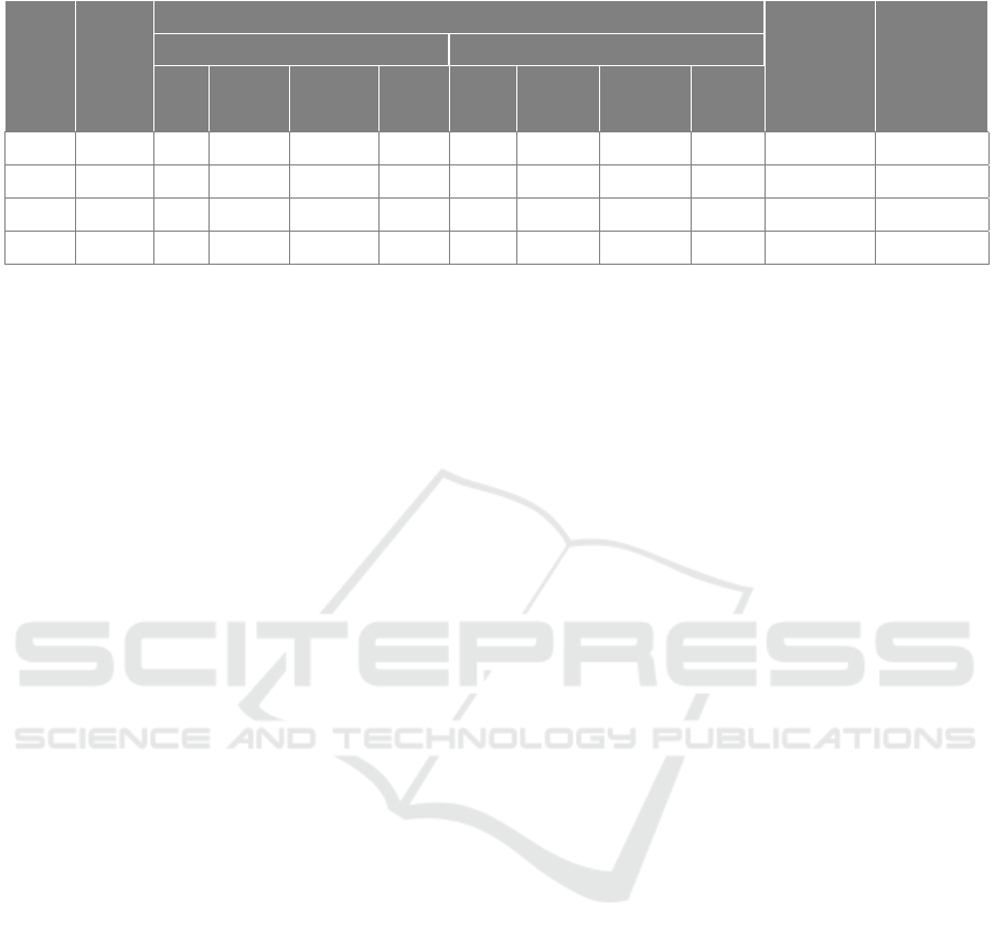
Table 1: Example of expected staffing actions in the FI occupation.
OCC–
LEVEL
HEAD–
COUNT
EXPECTED STAFFING
TOTAL
TURNOVER
(RATE)
TURNOVER
HISTORY
INFLOW OUTFLOW
HIRE PROMO DEMOTE TRANS
LEAVE
DEPT
PROMO DEMOTE TRANS
FI01 108 17.0 - 0.0 4.6 10.3 9.8 - 1.6 21.7 (20%) 10% - 39%
FI02 189 14.8 9.8 0.0 1.9 16 9.2 0 1.4 26.6 (14%) 6% - 31%
FI03 147 5.9 9.2 0.3 1.5 14.2 2.5 0 0.2 16.9 (11%) 4% - 22%
FI04 49 2.1 2.5 - 0.0 3.7 - 0.3 0.6 4.6 (9%) 5% - 17%
10 APPLICATION
Table 1 presents a small subset of a staffing analysis
conducted in DND. It shows expected staffing flows
for the four levels of the Financial Management (
FI)
occupation. The flows are broken down into hires,
promotions, demotions, transfers, and departures. As
this is based on an equilibriummodel, the sum of all
inflows equals the sum of all outflows – this sum is
highlighted as the total turnover. Turnover is an
indication of the number of staffing actions that will
need to be performed by Human Resources staff – it
is thus useful to the allocation of personnel
management resources. Turnover, and its
components also describes the dynamics of an
occupation, and is related to its health. Very high or
very low rates would warrant management attention,
and potentially, corrective measures.
Essentially, the method described in this paper
takes large quantities of historical Human Resources
data, and derives the personnel flows that would be
expected if the workforce were at equilibrium. These
flows describe the workforce’s dynamics, and Table
1 then presents these flows in a way that can be
readily assimilated by Human Resources Planners.
Some of the values in Table 1 can be broken down
further. In particular, transfer inflows (respectively
outflows) lump together all the transfers from
(respectively to) all other occupations. But the
specific origins and destinations of transfers would be
of interest to Human Resource Planners. Similarly,
promotions and demotions include ordinary moves
between adjacent levels, but also cases where an
employee skips one or more levels in changing
position (e.g. double promotions). Another
breakdown that can be of interest is the separation of
retirements from other sources of attrition, which can
be estimated based on the historical split. In DND,
highlighting how many of the hires are Canadian
Armed Forces Veterans is also a relevant concern.
Such breakdowns of the values in Table 1 are
normally reported in additional supporting tables.
Table 1 also reports a turnover history in the right-
most column. This is the range of turnover rates that
have been observed in past years. We have found that
reporting the turnover history provides empirical
context regarding the possible variability of
outcomes, in lieu of a derived confidence interval.
11 CONFIDENCE
This paper presents a method for deriving expected
staffing flows within a workforce. As with any
prediction, this must be accompanied by some
measure of the confidence that we have in the result.
The difficulty in this case is the absence of sufficient
historical data to bound the prediction. The values of
,
,
and
,
are based on annual historical
observation, but structural shifts in the workforce
generally means that data from more than a few years
ago is unlikely to be representative of the present or
future. Thus, we cannot directly observe historical
distributions of
,
,
and
,
that could be used to
derive reliable prediction intervals for the forecasted
staffing flows.
An alternative would be to fit a theoretically
justifiable probabilistic models of
,
,
and
,
with
the limited historical data that are available. Then,
the distributions of
,
,
and
,
could determine
prediction intervals for the reported equilibrium
staffing flow estimates. Substantial analysis would
however be required before this kind of probabilistic
model could be correctly employed.
The derivation of appropriate prediction intervals
to accompany the staffing flow estimates presented in
this paper will be an area of future work. For the time
being, we believe that historical ranges in the flows
provide reasonable bounds for our expectations of
ICORES 2019 - 8th International Conference on Operations Research and Enterprise Systems
210

future variability, and so this is what we have been
reporting.
12 PRACTICAL
CONSIDERATIONS
In practice, one of the most time consuming tasks in
the application of the presented method has been the
identification of historical exceptions that must be
ignored in deriving the values of
,
,
and
,
. In
the past, many events have taken place that should be
excluded in equilibrium staffing analyses. For
example, in the DND, entire units have been
transferred to other government departments, and
some occupations have been restructured, or split
from others, resulting in spikes in observed attrition
or transfers. However, there has been no centralized
record keeping of such changes. Careful outlier
detection of the historical record has been necessary
to identify the anomalies in the data record.
Another practical consideration has to do with the
many very small occupation-levels in the Department
of National Defence. It is unreasonable to model
staffing actions in very small occupations where the
historical record is insufficient to accurately describe
typical flow rates. Also, in very small occupations,
future events will not be averaged out over enough
individuals to be predictable. Ignoring the small
occupation-levels is not necessarily the best option.
First, Human Resources Planners might prefer a poor
estimate to none at all, but also, modelling the larger
occupation-levels still requires consideration of their
interactions with the smaller ones. The solution is to
aggregate select occupation-levels, such as
combining adjacent levels of an occupation. This is a
delicate task, as the small occupation-levels should
only be aggregated with similarly-behaving ones.
In order to determine when smaller occupation-
levels should be aggregated, an understanding of the
relationship between headcount and the width of
prediction intervals around occupation-level
estimates will be helpful. We would then keep
aggregating until the confidence intervals become
sufficiently narrow. So far, we have used 10 years of
historical data, and groupings of no less than 10
employees – giving a minimum of 100 employee-
years per segment. This is certainly on the low end
of statistical relevance. Until a characterization of
model confidence can be completed, we believe that
reporting the historical ranges in staffing flows will
provide sufficient context.
13 CONCLUSION
This paper presented a method that takes historical
staffing data as input, and derives expected
equilibrium staffing flows that have been valuable to
Human Resource Strategic Planning in Canada’s
DND. The expected flows can inform the allocation
of Human Resource capacity to process staffing
actions, and can also contribute to assessments of
occupational health by flagging occupation-levels
with unusually high or low flows.
REFERENCES
Bartholomew D.J., Forbes A.F. and McClean S.I., 1991.
Statistical techniques for manpower planning, John
Wiley and Sons. Chichester, United Kingdom, pp. 7-8.
Bartholomew D.J., 1969. A Mathematical Analysis of
Structural Control in a Graded Manpower System,
California University, Berkley, Ford Foundation
Program for Research in University Administration.
Available at:
https://files.eric.ed.gov/fulltext/ED080084.pdf
Calitoiu, D. and Vincent, E., 2017. Logistic Regression
Model for Attrition in DND Civilian Employees
(Director General Military Personnel Research and
Analysis Scientific Report DRDC-RDDC-2017-R177).
Defence Research and Development Canada, Ottawa,
ON.
Doumic, M., Perthame, B., Ribes, E., Salort, D. and
Toubiana, N., 2016. Toward an Integrated Workforce
Planning Framework using Structured Equations,
European Journal of Operational Research, 262(1), pp.
217-230. Elsevier. Available at: https://hal.inria.fr/hal-
01343368/document
Georgiou, A.C., 1999. Aspirations and Priorities in a Three
Phase Approach of a Nonhomogeneous Markov
System, European Journal of Operational Research,
116(3), pp. 565-583. Elsevier.
Fang, M. and Bender, P., 2011. Analyzing Changes in
Attrition of the Canadian Forces, In: MS 2011,
Modelling and Simulation Symposium, Calgary,
Canada.
Fang, M. and Bender, P., 2008. Canadian Forces Attrition
Forecasts – What One Should Know, (Centre for
Operational Research and Analysis Technical
Memorandum DRDC CORA TM 2008-60). Defence
Research and Development Canada, Ottawa, ON.
Available at:
http://cradpdf.drdc.gc.ca/PDFS/unc85/p531551.pdf
Filinkov, A., Richmond, M., Nicholson, R., Alshansky, M.
and Stewien, J., 2011. Modelling Personnel
Sustainability: A tool for Military Force Structure
Analysis, Journal of the Operational Research Society,
62(8), pp. 1485-1497. Springer.
Marquez, W. and Nelson, A., 1996. Total Army Personnel
Life Cycle Model: Development of a General Algebraic
Determining Equilibrium Staffing Flows in the Canadian Department of National Defence Public Servant Workforce
211

Modeling System Formulation (Study Report 96-07).
U.S. Army Research Institute for the Behavioral and
Social Sciences, Alexandria, VA, USA. Available at:
http://www.dtic.mil/dtic/tr/fulltext/u2/a315220.pdf
Mitropoulos, C.S., 1983. Professional Evolution in
Hierarchical Organizations, European Journal of
Operational Research, 14(3), pp. 295-304. Elsevier.
Okazawa, S., 2013. A Discrete Event Simulation
Environment tailored to the needs of Military Human
Resource Management, in WSC’13, 2013 Winter
Simulation Conference: Simulation: Making Decisions
in a Complex World, Washington, DC, USA. IEEE
Press, pp. 2784-2795. Available at:
https://ieeexplore.ieee.org/document/6721649/
Okazawa, S., 2007. Measuring Attrition Rates and
Forecasting Attrition Volume (Centre for Operational
Research and Analysis Technical Memorandum DRDC
CORA TM 2007-02). Defence Research and
Development Canada, Ottawa, ON. Available at:
http://cradpdf.drdc.gc.ca/PDFS/unc66/p527519.pdf
Zegers, A. and Isbrandt, S., 2010. The Arena Career
Modelling Environment – A New Workforce
Modelling Tool for the Canadian Forces. In: SCSC’10,
Summer Computer Simulation Conference, Ottawa.
Society for Modelling and Simulation International.
ICORES 2019 - 8th International Conference on Operations Research and Enterprise Systems
212
