3D Image Deblur using Point Spread Function Modelling for

Optical Projection Tomography

Xiaoqin Tang

, Gerda E. M. Lamers

and Fons J. Verbeek

1,2

Leiden Institute of Advanced Computer Science, Leiden University, Niels Bohrweg 1, Leiden, Netherlands

Institute of Biology Leiden, Leiden University, Sylviusweg 72, Leiden, Netherlands

Keywords: 3D Imaging, Point Spread Function, Optical Projection Tomography, Magnification, Deblur.

Abstract: Optical projection tomography (OPT) is widely used to produce 3D image for specimens of size between

1mm and 10mm. However, to image large specimens a large depth of field is needed, which normally results

in blur in imaging process, i.e. compromises the image quality or resolution. Yet, it is important to obtain the

best possible quality of 3D image from OPT, thus deblurring the image is of significance. In this paper we

first model the point spread function along optical axis which varies at different depths in OPT imaging

system. The magnification is taken into account in the point spread function modelling. Afterward,

deconvolution in the coronal plane based on the modelled point spread function is implemented for the image

deblur. Experiments with the proposed approach based on 25 3D images including 4 categories of samples,

indicate the effectiveness of quality improvement assessed by image blur measures in both spatial and

frequency domain.

1 INTRODUCTION

1.1 Background: 3D Image

Deconvolution

In biomedical research, i.e. disease and drug research,

optical techniques allow efficient and high-resolution

imaging of animal cell, tissues, organs and organisms.

Compared to 2D imaging, 3D imaging provides more

structural and comprehensive information, producing

more reliable and convincing evidence for research.

Optical projection tomography (Sharpe et al.,

2002), is a typical optical 3D imaging technique for

objects at tissue-, organ- and organism-level in the

magnitude range of millimeters, thereby filling a gap

between confocal and computational tomography

imaging in the resolution range. A point object

located within the DOF of the optical system is

considered to be in focus, but not necessarily at an

optimal focus. Beyond the DOF, the object is out of

focus (Walls et al., 2007). Depth of field (DOF) is

defined as a double fan symmetric around the focal

plane. For OPT imaging and reconstruction, the DOF

is expected to be large enough to contain as much of

the sample as possible. In this manner the parts of the

sample located in the DOF will result in an image

more or less in focus. However, according to previous

studies (Walls et al., 2007, NcNally et al., 1999), large

DOF subsequently produces image blur and results in

low in-focus image quality. In this paper the image

quality is also referred to as image resolution

according to some literatures. The trade-off between

DOF and image quality should be considered when

selecting lens for an OPT imaging system. A lens

with small numerical aperture (NA) will produce

large DOF, allowing imaging of larger samples but it

results in a relatively blurred image.

One typical way to improve the image quality to

the best resolution is applying deconvolution to the

raw tomography 2D images by using a constant

theoretical or experimental point spread function

(PSF). However, this approach is not strictly suitable

for OPT images; the raw OPT images normally

integrate the sample information of different depths

within a wide field. The imaging PSF within the field

varies at different depths along the optical axis.

Considering this variation of the PSF makes

deconvolution of 3D image more feasible and

promising. A 3D image is reconstructed from the

OPT images which are obtained by rotating the

specimen and acquiring a series of wide-field images

at regular angular intervals. This is accomplished

over a full revolution of the specimen. The filtered

Tang, X., Lamers, G. and Verbeek, F.

3D Image Deblur using Point Spread Function Modelling for Optical Projection Tomography.

DOI: 10.5220/0007237700670075

In Proceedings of the 12th International Joint Conference on Biomedical Engineering Systems and Technologies (BIOSTEC 2019), pages 67-75

ISBN: 978-989-758-353-7

back-projection (FBP) algorithm is typically used for

3D image reconstruction (Kak et al., 2001) in this

case. Deconvolution implemented on the

reconstructed 3D image is regarded as 3D image

deconvolution.

According to Chen et al., (2012), OPT is typically

undertaken with specimens that extend beyond the

confocal parameter i.e. the Rayleigh range, of the

imaging lens. Therefore, the tangential resolution of

the reconstructed 3D image decreases away from the

focal plane radially. When the focal plane is

coincident with the center of rotation (COR), the

tangential resolution decreases centered on the COR

in a radial-symmetrical fashion. For an imaging

system with a focal plane located away from the COR

the decrease in resolution is more complicated but the

highest resolution is still found around the focal

plane. The focal plane in the reconstructed slice

corresponds to a circle centered around the COR,

rather than a point coincident with the COR. This

subsequently appears as a cylindrical surface in the

3D image centered by the COR.

The aim of our contribution lies in deblurring the

OPT 3D image (improving the visual resolution) by

means of deconvolution, based on the modeled PSF

of the imaging system. This will, for large samples

with focal plane being at or away from the COR,

recuperate the imperfections of 3D image resulting

from the imaging system. The method in the

modelling of PSF will be explained in Section 2 and

the qualitative and quantitative image comparison

will be presented in Section 3. In section 4 we will

present our conclusions.

1.2 Related Works

Accounting for the trade-off between large DOF and

high resolution, previous studies have proposed

several methods to solve the problem. One approach

is choosing a high NA lens to acquire a high-

resolution image and combining multiple focal planes

in a simultaneous manner (Chen et al., 2013) or

scanning the focal plane through the sample (Miao et

al., 2010). These multiple focal plane approaches

solve the issue of narrow DOF, but the mechanism of

multiple measurements and scanning increases the

acquisition time and the complexity of the imaging

system. Considerably another direction is to use a

reasonable NA lens and deblur the image by

employing a deconvolution or filter on images before

or after reconstruction. Walls et al., (2007) first

applied the frequency-distance relationship (FDR)

(Xia et al., 1995) to OPT. The corresponding filter

was implemented on the sinogram before

reconstruction. The quality of the 3D image can be

further improved with weighted filtered back

projection (WFBP) (Darrell et al., 2008); this is done

by considering the intensity distribution of multiple

fluorescent spheres of known size along the optical

axis. But the implementation of evenly placing each

sphere along the optical axis is rather difficult to

achieve. Chen et al., (2012) proposed a way to

determine the modulation transfer function (MTF)

that contributed to MTF-mask filter and MTF-

deconvolution filter in the reconstruction process.

The former filter significantly reduced the artifacts

produced by sparse projection but the latter filter had

limited improvement on tangential image resolution.

Additionally, a spatial-invariant experimental PSF

was investigated by McErlean et al., (2016) in order

to improve the spatial resolution. However, spatial-

invariance of the PSF is not completely convincing

for OPT. Most recently, a new deconvolution

approach based on the reconstructed 3D image was

proposed by Horst et al., (2016). In their approaches

the PSF was modelled and as such they achieved

significant improvement on the reconstructed slice.

Nevertheless, they focused on the deconvolution of

vertically independent slices and omitted the PSF

diffractions along the optical axis that concerns the

interaction of different slices.

In this paper, we contribute by modeling the

experimental PSF of a single sphere along optical

axis, thereby considering the interaction of

contiguous slices from the reconstructed volume. At

the same time, the magnification is taken into account

in an experimental manner. As discussed in section

1.1, the tangential resolution of the OPT 3D image

slice decreases radially around the focal plane.

Theoretically the best resolution of the reconstructed

3D image can be achieved by combining all the

coronal deconvolutions of different angles. The

coronal deconvolution means deconvolving the 3D

image with the PSF slice by slice in the coronal plane

along its depth axis. This depth axis is parallel to

optical axis of the modelled PSF. We only implement

the coronal deconvolution in 2 opposite angles, i.e.

the reconstructed 3D image and its opposite sample at

180° centered by the COR, in parallel considering the

enormous time consumption of 3D matrix rotation in

N angles and the symmetry of the focal plane. When

the focal plane is off the COR during imaging

process, the shift is accounted for by a shift in PSF

modelling. This paper focuses on the presentation of

the concept of PSF modeling and coronal

deconvolution on 3D OPT data, accompanied by

some initial experimental results based on 25 3D

images including 4 categories of samples. Further

BIOIMAGING 2019 - 6th International Conference on Bioimaging

evaluations on a larger number of data are the topics

of our current research.

2 MATERIALS AND METHOD

2.1 The OPT Imaging System

Our homemade OPT imaging system consists of a

Leica MZ16 FA stereomicroscope with a Plan 0.5×

and 135mm working distance objective lens (Leica

10446157). Images are acquired by a 1360×1036

pixel Retiga Exi CCD with a well size of

6.45μm×6.45μm and saved as 12-bit tiff-files. A full

revolution results in a 1.13Gb tiff-file. The

acquisition is accomplished by a rotation of the

specimen driven by a stepper unit; the stepper moves

0.9°per step and it results in 400 images per

revolution. The OPT imaging system has two

modules: for bright-field imaging the specimen is

illuminated with a LED and for fluorescence imaging

a 100W mercury lamp is used in combination with a

filter-block (GFP1, Texas Red).

2.2 Sample Preparation of a Single

Fluorescence Sphere

To image the specimens in the range of several

millimeters small-valued NA (effective NA:

0.0105~0.0705) lens is used to obtain the large DOF

in our OPT imaging system. The resolution of an

optical system is defined as the minimum distance 

at which two separate points can be distinguished as

individuals. According to the Rayleigh criterion

  for a circular aperture where

 is the emission wavelength, the minimum

size of the experimental fluorescence sphere is

supposed to be in the range between 4.40 and

29.57. To make it visible in the image the sphere

size is supposed to exceed this range. In our case, we

choose the green fluorescent protein (GFP) sphere of

size and diluted it to a concentration of 360

.

To image and model the PSF along optical axis

we have developed an injection-based protocol to

place the spheres into agarose as follows:

 1% low melting point (LMP) agarose, cool down

to ~37;

 Drill cylindrical agarose shapes when it is semi-

solidified in a petri dish;

 Inject the diluted spheres into the outer wall of the

agarose along a line parallel to the central axis,

preferably with a small size syringe. In our case a

0.5 syringe is used with a needle length of

13mm and diameter of 0.29mm, as shown in

Figure 1;

Figure 1: The injection protocol with green spots indicating

the injection position where fluorescence spheres may

occur. The cylinder corresponds to the shape of the agarose.

 Keep the agarose at 4 until it is fully solidified

(~3 hours);

 Clear the sample with 70%, 80%, 90%, 96%,

100% ethanol, 100% ethanol: BABB (benzyl

alcohol: benzyl benzoate = 2: 1) = 1: 1 and BABA.

Our goal is to acquire the images of a single sphere

placed at different depths along optical axis.

Therefore, randomly sprinkling the spheres into the

agarose in a traditional way is not feasible. The main

reason is that there may be interactions and overlap

between different spheres either at the same or

different depths. This makes the extraction of the

single sphere image difficult or even impossible. The

images of each single sphere at different depths are

acquired by means of sample rotation. Each rotation

corresponds to a different depth in the OPT imaging

system. The straight-like sphere injection method in

of our protocol significantly reduces the probability

of overlapping between different spheres. In this way

the images of the same sphere in a full revolution can

be easily and efficiently acquired. The OPT imaging

system and environment is configured as explained in

(Tang et al., 2017).

2.3 PSF Modelling Concerning

Different Magnification

For our experiments a full revolution of 400 images

of the single GFP sphere are acquired. In Figure 2 the

processes of sphere image acquisition and PSF

modelling are presented. In Figure 2(a) and (b), the

green dot represents the sphere and the red arrow

indicates the sphere rotation. The excitation and

emission beams are regarded to be parallel,

demonstrated as blue and green beams in Figure 2(a).

For PSF modelling, the focal plane is set at the COR.

The 3D image whose focal plane is shifted from the

COR, requires an equal shift in the PSF. With the

protocol (cf. section 2.2) the physical rotation radius

of the sphere 



can be easily measured. To this end,

we first measure the radius of the cylindrical agarose





and image it in the bright-field mode with small

3D Image Deblur using Point Spread Function Modelling for Optical Projection Tomography

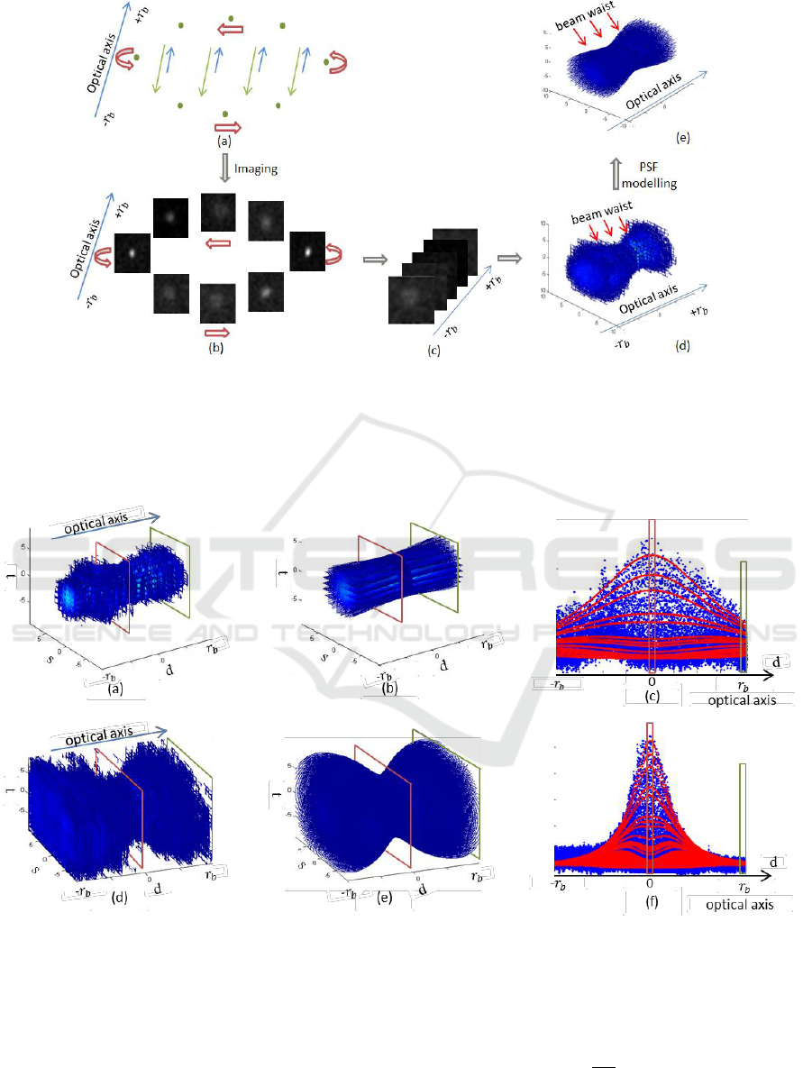
Figure 2: Image acquisition and PSF modelling of a single GFP sphere. (a) The light path of the OPT imaging system that

passes through GFP spheres (green dots). The excitation beams and emission beams are separately shown in blue and green

arrows. (b) Images of the single sphere acquired at different angles. (c) Images of the single sphere stacked according to the

defocus. Half rotation with defocus from 



to



is required, in our experiment



 as calculated from Eq. (1).

(d) The experimental and discrete PSF with defocus from 



to



. (e) The modelled and continuous PSF with defocus

from 



to



Figure 3: PSF modelling along the optical axis. (a), (d) Experimental PSFs acquired from images at magnification of 12.5

and 25.0. (b), (e) The corresponding modelled PSFs using Eq. (4) and Eq. (5). All the voxels of experimental data in (a)

and modelled data in (b) are respectively transformed to blue and red dots in 1D functional in (c) to visualize the modeling

performance. The vertical axis in (c) displays the intensity that corresponds to the voxel intensity in (a) and (b). Similarly,

voxels in (d) and (e) are transformed to the data in (f).

exposure time. In the same experimental

environment, the sphere is afterwards imaged in the

fluorescence mode. 



is calculated by Eq. (1).















 



(1)

BIOIMAGING 2019 - 6th International Conference on Bioimaging

with 



representing the rotation diameter of the

sphere in the tomogram, achieved by measuring the

distance of two opposite sphere centers that are both

in focal plane. 



is the diameter of the cylindrical

agarose in the bright-field image. Dividing 



by 100

rotations, the distance of each rotation along optical

axis is determined. In our case the measured





, 







, producing 



mm.

Therefore, the physical distance of two adjacent

rotations along optical axis is approximately.

According to convention the imaging PSF is

assumed as a focused Gaussian-like beam:

















 





 









(2)

where is the beam waist (Figure 2)given by:



















 











(3)

With 



the Gaussian beam waist defined as the 

value of the field amplitude in focus (van der Horst et

al., 2016),  the emission wave length of fluorescence

spheres and  the defocus along optical axis. For a

specific magnification, 



is constant, but it varies

when imaging with different magnifications.

Additionally, in Eq. (2) and Eq. (3) the beam waist

 is typically regarded as the standard deviation of

the Gaussian model in previous studies (van der Horst

et al., 2016). Different from the Gaussian model in

(van der Horst et al., 2016), we generalize the model

by employing parameter



, 



and 



as:





















 





 













 



(4)

Instead of equalizing the beam waist and standard

deviation as described in (van der Horst et al., 2016)

and (Kogelnik et al., 1966), we investigate the

relationship between them by multiplying a

parameter  with beam waist, considering different

magnifications.









 









 











(5)

To relate the beam waist in focus 



as well as the

parameter a to the magnification, 6 magnifications

i.e. 12.5, 15.0, 17.5, 20.0, 22.5, 25.0,

are configured to acquire the images of the same

sphere. The magnifications are obtained through

zooming. The magnification of 12.5 approximately

corresponds to the minimum magnification that

renders the sphere visible in our experiment, while

25.0 approximates to the maximum magnification

that confirms that a full revolution of the sphere

remains in the field of view (FOV). The PSF of each

magnification is modelled by creating an

optimization problem and solving it with least square

curve fitting. The overall fitting error of the 6

experimental PSFs is 5.00%. The experimental PSFs

acquired from images with magnification of 12.5

and 25.0 are shown in Figure 3 (a) and (d)

respectively. The color of the voxel indicates the

intensity of PSF response. (b) and (e) represent the

modelled PSFs of the two magnifications. Voxels in

3D space are converted to a 1D space with horizontal

axis approximating the optical axis and vertical axis

displaying the intensity. The 3D voxels on the slice in

(a) and (b) match the 1D points in the box in (c)

according to the same color. The experimental PSF

differentiation between two magnifications is evident

in (a) and (d). By transforming the 3D space to 1D

functional, we can intuitively visualize the

distribution of the experimental PSF (blue dots) and

the modelled PSF (red dots), as well as showing the

differences between them.

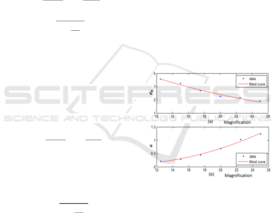
Figure 4: Fitting of 



and the parameter a estimated from

6 magnifications. 



is fitted by exponential function as

shown in (a) while a is fitted by quadratic function in (b).

The parameters for our modelling







and 



have proved to be constant regardless of

magnifications: 



, 



 and 





  



. The beam waist 



and parameter a

relevant to the 6 magnifications are estimated as

depicted in Figure 4. To minimize the fitting error on

the observed data, the parameters are fitted as an

exponential and a quadratic function respectively by

using Eq. (6) and Eq. (7), with  representing

magnification and 



to 



being the parameters.

3D Image Deblur using Point Spread Function Modelling for Optical Projection Tomography









 







(6)









 



 



(7)

The PSF of any 3D image between and

along optical axis can be modelled as depicted in

section 2.3. The modeling is implemented with the

focal plane set at the COR. However, in most imaging

cases the focal plane is not in line with the COR.

Consequently, the modelled PSF will be shifted along

the optical axis by the same shift as the focal plane.

Besides, the length of the PSF along optical axis is

determined by the size of 3D image and the

resolution, because in FBP 3D reconstruction each

voxel in the 3D image corresponds to each pixel in

the 2D images. The NA is the effective value

achieved from interpolation relating to the

magnification. The relationship between effective

NA and magnification can be found in the product

manual of the Leica objective lens.

2.4 Deconvolution of 3D Images in

Coronal Plane

The modelled PSF consists of multiple 2D Gaussian

patterns along optical axis. Therefore, the 3D image

can be deconvolved slice by slice along its depth axis

that is parallel to the optical axis. As the slices are

coronal sections, the deconvolution is implemented

on the 3D image  in the coronal plane as follows:









 



(8)

R is the reconstructed 3D image with the depth axis d

parallel to the optical axis of the PSF.  stands for

the operation of deconvolution. Considering the

shifted focal plane and the reconstruction symmetry,

deconvolution of



, the opposite view of R projected

along d, is executed by applying Eq. (9).





















 







(9)

The transform from  to 



is conducted by a matrix

rotation of  centered by the COR. The 3D image

with the deconvolution is then achieved by combining

 and  back rotation of



3 EXPERIMENTS

3.1 Image Comparison of

Deconvolution

With respect to the magnifications, the experiments

were conducted on images at 2 different

magnifications. One is a zebra finch embryo in

fluorescence mode with magnification 13.83 and

focal plane shifted by. Considering the

resolution limit and the 3D image size, the calculated

defocus of the PSF along the optical axis ranges

from to. The deconvolution is

performed using Lucy-Richardson algorithm with 10

iterations. The result for the coronal slice is shown in

Figure 5 (b) and for the horizontal slice in Figure 5

(d). The corresponding slices without deconvolution

are displayed in Figure 5 (a) and (c). The comparisons

of intensity profile along a line with (red) and without

(blue) deconvolution are presented in (e) and (f)

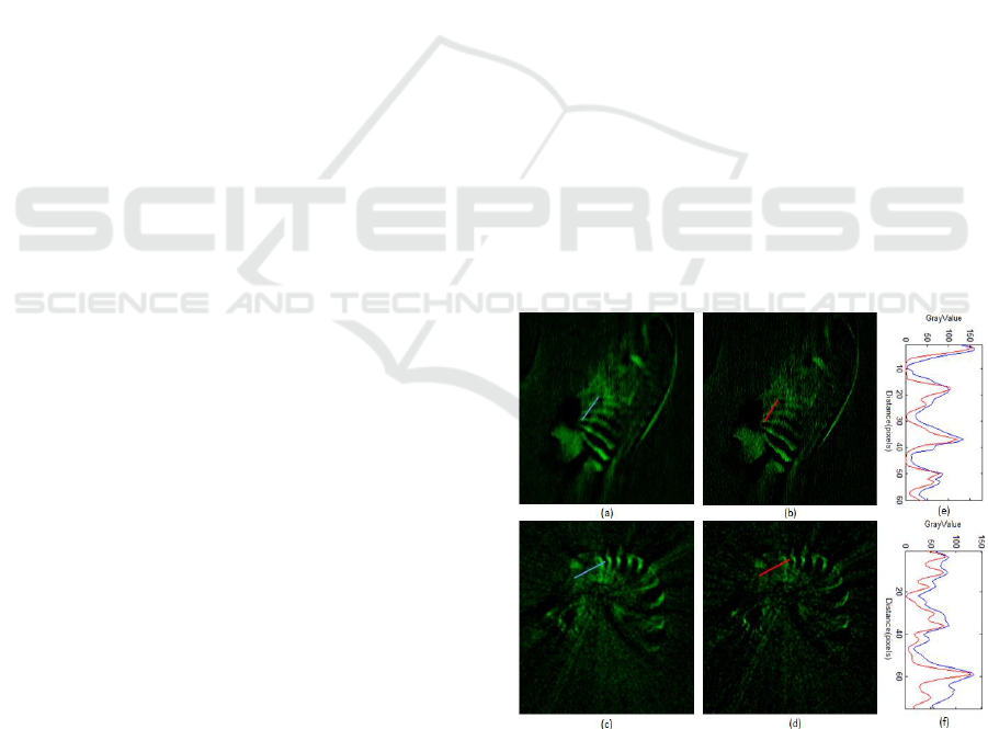
respectively. In Figure 6 another sample is depicted.

This is a sample from a 3dpf batch of zebrafish larvae.

The magnification and the shifted focal plane are

separately 49.98 and -0.5mm, with the computed

defocus of PSF as between 

and. Figure 6 (a) and (b) are the slices

before deconvolution in two orthogonal planes, while

By visually comparing (c) and (d) we conclude that

the performance in horizontal plane is as good as it is

in coronal plane. This means that deconvolution in the

coronal plane simultaneously improves the quality of

the image in the horizontal plane. From a comparison

of the quantitative intensity profile for each colored

line, we state that the proposed deconvolution

sharpens and refines the 3D reconstructed images. It

enhances the strong signals and makes the intensity

profile more distinct.

Figure 5: Deconvolution results. (a) The coronal slice of the

3D zebra finch with obvious blur around the ribs. (b)

Distinct texture appears around the ribs after the

deconvolution. (e) The comparison of intensity profiles

along a line in (a) and (b). (c) and (d) The horizontal slice

comparisons with the line intensity profiles shown in (f).

BIOIMAGING 2019 - 6th International Conference on Bioimaging

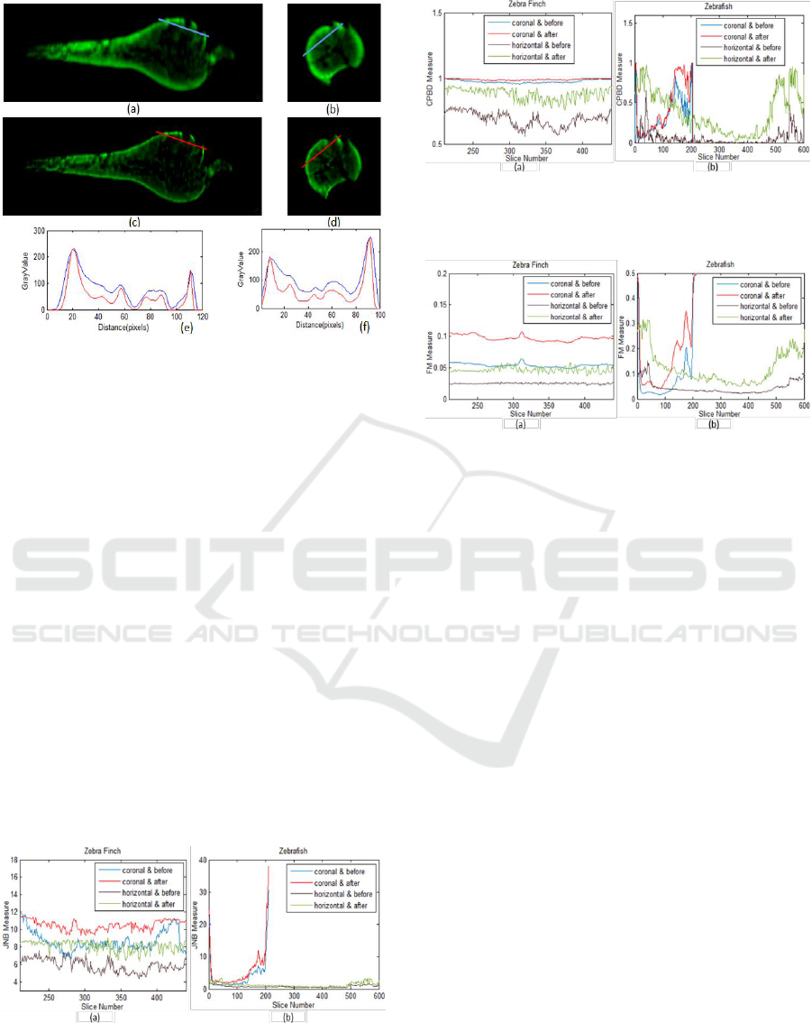
Figure 6: Coronal and horizontal slices of 3D zebrafish

before ((a) and (b)) and after ((c) and (d)) deconvolution.

The deconvolution highlights the strong signals and makes

the texture more visible. The figure below (a) and (c)

compares the intensity profile of the same line before

(labelled as blue) and after (labelled as red) deconvolution,

so does the figure below (b) and (d).

3.2 Image Blur Measurement on Slices

To quantify the image blur of each slice, 3 metrics

from literatures, i.e. the just noticeable blur (JNB)

measure (Ferzli et al., 2009), the cumulative

probability of blur detection (CPBD) measure

(Narvekar et al., 2009) and the frequency measure

(FM) (De et al., 2013) are employed to evaluate the

performance. Both the JNB and CPBD measure

acquire sharpness metric by detecting and quantifying

the blur in the spatial domain. Different from JNB and

CPBD, the FM measure quantifies the sharpness in

the frequency domain with an easier and more

efficient approach. All the three metrics characterize

the sharpness of an image, so the measure increases

at improved image quality.

Figure 7: (a) JNB measure on the zebra finch data with

magnification 13.83. (b) JNB Measure on the zebrafish

data with magnification 49.98. Coronal and horizontal

are the two orthogonal planes displaying the 3D image.

Figure 8: (a) CPBD measure on the zebra finch with

magnification 13.83. (b) CPBD Measure on the zebrafish

with magnification 49.98.

Figure 9: The FM before and after deconvolution on the two

3D image data. (a) FM measure on the zebra finch with

magnification 13.83. (b) FM Measure on the zebrafish

with magnification 49.98.

While experiments in section 3.1 give us a

qualitative comparison between the deconvolved

slice and non-deconvolved slice, in this section we

quantitatively look into all the slices in different

orthogonal planes with the three image sharpness

measurements (i.e. JNB, CPBD and FM). From

Figure 7 to Figure 9 we can see that, no matter what

measure is used, the deconvolved slices in both planes

have higher measurement values compared with the

image slices without deconvolution. This means that

on all slices, the deconvolution deblurs the images

and significantly improves the image quality.

3.3 Quantitative 3D Image Quality

Improvement of Deblur

To further quantify the deblur of the deconvolution

results on the original reconstructed 3D data across

the planes, we present the 3D image quality

improvement criterion of deblur as 



in Eq. (10).

Improvement in three orthogonal individuals are

combined and encoded as a whole and each of them

are represented as Eq. (11) to Eq. (13).

3D Image Deblur using Point Spread Function Modelling for Optical Projection Tomography

Table 1: 3D image quality improvement of 10 zebrafish

embryos based on JNB Measure.

0.16

0.21

0.15

0.21

0.29

0.24

0.22

0.16

0.20

0.25

PSF

1.35

2.10

1.41

3.23

1.54

1.50

1.37

1.45

1.70



-- Gaussian-based blind deconvolution. PSF

-- PSF based modelling

deconvolution. 10 zebrafish embryos correspond to 01-10 with age ranging

from 3dfp to 7dfp. Magnification for 01-05 is 24.98 while for 06-10 is

22.45.

Table 2: 3D image quality improvement of 6 zebrafish brain

based on JNB Measure.

0.25

0.29

0.26

0.24

0.01

0.21

PSF

0.41

0.49

2.55

0.17

1.15

1.20

 6 zebrafish embryo brains correspond to 01-06 with age ranging from

6dfp to 7dfp. Magnification for 01-02 is 20.98 while for 03-06 is

15.98.

Table 3: 3D image quality improvement of 7 chicken heart

based on JNB Measure.

0.24

0.16

0.19

0.26

0.27

0.18

0.32

PSF

0.93

0.49

0.29

1.15

0.49

0.38

1.07

 7 chicken embryo hearts at different stages correspond to 01-07.

Magnification for 01 is 15.00 ,while for 03-06 is 11.75 and 07 is

10.00.































 





































(10)













 











(11)













 











(12)













 











(13)

Where 





and 





are the ith deconvolved and

original reconstructed slice in x plane respectively.

By employing the image quality improvement of

deblur 



, deconvolution performance of two

different methods on the same data turns to be

comparable.

We here applies our deconvolution method to 23

more 3D data, which contains 3 categories of samples

i.e. zebrafish embryo, zebrafish embryo brain and

chicken embryo heart. They are in different stages

and are acquired at different magnifications. It is

important to know that all the measurements in this

paper cannot assess the image blur across different

data, but it provides us with a comparative evaluation

of image deblur on the same data. Taking advantage

of this, we compare the presented deconvolution

method with the most commonly used Gaussian-

based blind deconvolution (Chan et al., (1998)). The

Gaussian kernel size is set to 7 for all slices. As the

most robust measurement among CPBD, JNB and

FM, JNB is employed to evaluate the image blur of

each slice. The results of the 3 categories of samples

are presented in Table 1 to Table 3. For all the 23 data,

our deconvolution approach outperforms the

Gaussian-based deconvolution, thereby indicating the

success of the method.

4 CONCLUSIONS

In this paper we have focused on 3D image deblur and

quality improvement, under the condition of the

limitation of small NA for imaging of large samples.

We investigated and modeled the PSF along the

optical axis, exploring the influence of magnification

on PSF. The sample of a single GFP sphere is

prepared with the protocol in section 2.2. The

experimental PSF is then modelled to deconvolve the

3D image in a coronal plane. A number of measures

for image blur are employed to convincingly evaluate

the performance of the deconvolution. They provide

quantitative information about how much

improvement is achieved. The overall

improvement



gives us a criterion to compare

image quality improvement regardless of different

data. All the experimental results including the image

comparisons and quantitative measures sustain the

effectiveness of the proposed PSF modelling and

deconvolution methodology.

The deconvolution results presented in this paper

represent a proof of concept. The datasets used in the

experiments are composed of 25 samples (i.e. 4

categories: zebrafish embryo, zebra finch embryo,

zebrafish brain and chicken heart). Regarding the

evaluation of performance on a large scale of dataset,

our data are far from perfect in terms of ‘large

dataset’. However, it presents a clear idea that our

model is not constrained by several samples, it also

works on many other types of objects or images. This

will help to explain its potential capability of

improving image quality on more 3D data, including

those from other OPT imaging systems, which is a

part of our current work. In the future we will take

BIOIMAGING 2019 - 6th International Conference on Bioimaging

more effort on further generalizing the model to other

imaging set-ups. In addition, the fluorescent sphere

used in the experiments is fix-sized. The effect of

sphere size on PSF modelling and deblur performance

will be investigated afterwards.

REFERENCES

Sharpe, J. et al., 2002. Optical projection tomography as a

tool for 3D microscopy and gene expression studies.

Science (80-. ), vol. 296, no. 5567, pp. 541–545, 2002.

Walls, J. R., Sled, J. G., Sharpe, J. and Henkelman, R. M.,

2007. Resolution improvement in emission optical

projection tomography. Phys. Med. Biol., vol. 52, no.

10, p. 2775.

McNally, J. G., Karpova,T., Cooper, J. and Conchello, J.

A., 1999. Three-dimensional imaging by deconvolution

microscopy. Methods, vol. 19, no. 3, pp. 373–385.

Kak, A. C. and Slaney, M., 2001. Principles of

computerized tomographic imaging. SIAM.

Chen, L. et al., 2012. Incorporation of an experimentally

determined MTF for spatial frequency filtering and

deconvolution during optical projection tomography

reconstruction. Opt. Express.

Chen, L., Andrews, N., Kumar, S., Frankel, P., McGinty, J.

and French, P. M. W., 2013. Simultaneous angular

multiplexing optical projection tomography at shifted

focal planes. Opt. Lett., vol. 38, no. 6.

Miao, Q., Hayenga, J., Meyer, M. G., Neumann, T., Nelson,

A. C. and Seibel, E. J., 2010. Resolution improvement

in optical projection tomography by the focal scanning

method. Opt. Lett., vol. 35, no. 20, pp. 3363–5.

Xia, W., Lewitt, R. M. and Edholm, P. R., 1995. Fourier

correction for spatially variant collimator blurring in

SPECT. IEEE Trans. Med. Imaging, vol. 14, no. 1, pp.

100–115.

Darrell, H. Meyer, K. Marias, M. Brady, and J. Ripoll.,

2008. Weighted filtered backprojection for quantitative

fluorescence optical projection tomography. Phys.

Med. Biol., vol. 53, no. 14, pp. 3863–81.

McErlean, C. M., Bräuer-Krisch, E., Adamovics,J. and

Doran, S. J., 2016. Assessment of optical CT as a future

QA tool for synchrotron x-ray microbeam therapy.

Phys. Med. Biol., vol. 61, no. 1, pp. 320–37.

van der Horst, J., and Kalkman, J., 2016. Image resolution

and deconvolution in optical tomography. Opt.

Express, vol. 24, no. 21, pp. 24460–24472.

Tang, X., van der Zwaan, D., Zammit,M., Rietveld, A., K.

F. D. and Verbeek, F. J., 2017. Fast Post-Processing

Pipeline for Optical Projection Tomography. IEEE

Trans. Nanobioscience, vol. 16, no. 5, pp. 367–374, Jul.

Kogelnik, H. and Li, T., 1966. Laser Beams and

Resonators. Proc. IEEE, vol. 54, no. 10, pp. 1312–

1329.

Ferzli, R. and Karam, L. J., 2009. A no-reference objective

image sharpness metric based on the notion of Just

Noticeable Blur (JNB). IEEE Trans. Image Process.,

vol. 18, no. 4, pp. 717–728.

Narvekar, N. D. and Jaram, L. J., 2009. An improved no-

reference sharpness metric based on the probability of

blur detection. IEEE Int. Work. Qual. Multimed. Exp.,

vol. 20, no. 1, pp. 1–5.

De, K. and Masilamani, V., 2013. Image Sharpness

Measure for Blurred Images in Frequency Domain.

Procedia Eng., vol. 64, no. Complete, pp. 149–158.

Chan, T.F. and Wong, C.K., 1998. Total variation blind

deconvolution. IEEE Transactions on Image

Processing, vol. 7, no. 3, pp. 370—375.

3D Image Deblur using Point Spread Function Modelling for Optical Projection Tomography