
Variation Number of Blades for Performance Enhancement for
Vertical Axis Current Turbine in Low Water Velocity in Indonesia
Madi, Shade Rahmawati, Mukhtasor, Dendy Satrio and Ahmad Yasim
Department of Ocean Engineering, Institut Teknologi Sepuluh Nopember, Surabaya 60111, Indonesia
Keywords: Vertical Axis Current Turbine, Number of Blades, Performance Enhancement, Low Water Velocity.
Abstract: Asosiasi Energi Laut Indonesia (ASELI) has provided the results of the ratification of the energy potential
of ocean currents in Indonesia amounting to 17,989 MW. This amount is very large considering that
Indonesia is classified as in low water velocity. The vertical axis current turbine is proposed by many
researchers because they have lower performance than the horizontal axis current turbine. So this study
proposes research to improve the performance of the vertical axis current turbine for low water velocity by
varying the number of blades. The type of blade NACA 63
4
021 chose because has good performance for the
vertical axis current turbine of Darrieus type. The model of the turbine is simulated by Computational Fluid
Dynamics (CFD) with variations of the number of blades namely, 3, 4, and 5. The totals of the statistic
element of meshing are 16,090, 167,020, and 174,375 at the number of blades 3, 4, and 5, respectively. The
inlet velocity set at 1.5 m/s and tip speed ratio (TSR) are 1.5, 2, and 2.5. The final results of this study show
that the blade numbers can improve the performance of the turbine model on all TSR ranges. The blades 4
and 5 are increased by 21.8% and 15% respectively from the blades 3 on TSR 2.5. The highest performance
is obtained by the number of blades 4 on TSR 2.5 with the value of the power coefficient (Cp) 0.26.
1 INTRODUCTION
One of the technologies that are usually used for the
current energy source is the turbine. The turbine is
the main equipment in addition to the generator
(Madi et al., 2019). Generally, the turbine that is
used in the world operated in the higher current
speed, such as in Columbia 1.5-2.5 m/s (Rawlings,
2008), Italy 2 m/s (Castelli et al., 2013), China 3-4
m/s (Jing, 2014), Korea 3 m/s (Quang Le et. al,
2014), and Australia 1.5-2 m/s (Marsh et al., 2015).
Whereas several potential locations in Indonesia are
classified in the low water velocity, they can only
achieve a maximum current speed of 1.39, 1.5, and
1.79 m/s at Riau strait, Boleng strait and Mansuar
strait, respectively (Mukhtasor et al., 2014; Satrio et
al., 2018). So, the turbine which already exists in the
world, cannot be applied in Indonesia.
Asosiasi Energi Laut Indonesia (ASELI) has
provided the results of the ratification of the energy
potential of ocean currents in Indonesia amounting
to 17,989 Megawatt (Mukhtasor et al., 2014). The
amount is very abundant considering that Indonesia
is classified as in the low water velocity. Therefore,
the turbine is needed that can be applied in the low
water velocity in Indonesia.
In general, the turbine consists of two based on
its rotating axis namely, the vertical axis current
turbine (VACT) and horizontal axis current turbine
(HACT) (Khan et al., 2009; Hydrovolts, 2006 and
Duvoy et al., 2012). The VACT can respond to any
flow direction, so the results of efficiency will
stable. Whereas the HACT only responds in one
flow direction, so the results of efficiency will not
stable (Kirke and Lazauskus, 2011; Zeiner, 2015;
Bachant and Wosnik, 2015; Satrio et al., 2016).
Therefore, this study case will focus on the design of
VACT.
Particularly, the VACT consists of two namely,
Darrieus type and Savonius type (Khan et al., 2009).
The turbine of the Darrieus type is higher efficiency
than the Savonius type. However, in practice, the
efficiency is still under the HACT. It is a challenge
for researchers in this research. This study case will
try to improve efficiency the VACT of Darrieus type
in the low water velocity, by varying the number of
blades 3, 4, and 5 (Fig. 1). The blades are simulated
by Computational Fluid Dynamics (CFD).
Madi, ., Rahmawati, S., Mukhtasor, ., Satrio, D. and Yasim, A.
Variation Number of Blades for Performance Enhancement for Vertical Axis Current Turbine in Low Water Velocity in Indonesia.
DOI: 10.5220/0010047900470053
In Proceedings of the 7th International Seminar on Ocean and Coastal Engineering, Environmental and Natural Disaster Management (ISOCEEN 2019), pages 47-53
ISBN: 978-989-758-516-6
Copyright
c
2021 by SCITEPRESS – Science and Technology Publications, Lda. All rights reserved
47
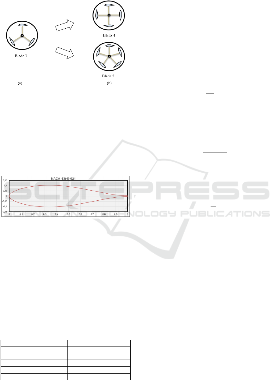
Figure 1: (a) Basic turbine, (b) variations turbine.
The type of blade NACA 63
4
021 is chosen for
this study because it is similar to the morphology of
humpback whales flippers (Fish and Battle, 1995).
The humpback whales are the most maneuverable of
other species and have a symmetric body so that
they will be stable and fast to catch prey (Johari et
al., 2007). The blade profile of NACA 63
4
021 in the
VACT of Darrieus type has a good performance
(Marsh et al., 2015). The profile of NACA 63
4
021
can be shown in Fig. 2.
Figure 2: The profile of NACA 63
4
021.
2 NUMERICAL SIMULATIONS
2.1 Turbine Geometry
Three types of turbine designs are simulated to
evaluate the influence of variations of the number of
blades. The turbine geometry (Table 1) is used based
on the published 3D CFD model data by Marsh et al
(2015). The turbine with three blades namely basic
turbine (Fig. 1a) is designed and simulated for
compared with the results of the 3D CFD model by
Table 1: Turbine Geometry.
Geometry Dimensions
Blade type NACA 63
4
021
Chord length (C) 0,065 m
Number of blades (N) 3, 4 and 5
Diameter of turbine (D) 0,914 m
Height of turbine (H) 0,686 m
Marsh et al (2015). After that, the variations turbine
(Fig. 1b) is designed and simulated to obtain the
influence of the performance of the turbine.
2.2 Key Performance Parameters
The performance parameters of the turbine blades
are investigated for this study namely, solidity (𝜎),
torque (𝑇), and power of the turbine (P
t
).
The solidity of the turbine is defined as the ratio
of rotor blade surface area to the frontal, swept area
that the rotor passes through (Li, 2010), where,
𝜎
(1)
where N is the number of blades, C is chord length
(m), and R is the radius of the turbine (m).
The torque of the turbine represents the torque
coefficient. The comparison of torque of the turbine
and hydrodynamic subsystem is called by the torque
coefficient (Ct), where,
𝐶𝑡
,
(2)
where p is the density of the water (998.2 kg/m
3
), A
is the turbine swept area (HxD), and V is current
velocity (m/s).
The power of the turbine represents the power
coefficient (Cp), where,
𝐶𝑝
(3)
where P
t
is the power mechanic of the turbine (watt)
and P
a
is the power kinetic of the water (watt).
The power of the turbine is obtained from the
value of the torque and the rotational speed, shown
in equation 4. Whereas the power kinetic is obtained
of available in the water (equation 5).
P
t
= T x ω
(4)
where ω is the rotational speed (rad/s) and T is the
torque of the turbine (N.m).
P
a
= 0,5 p A V
3
(5)
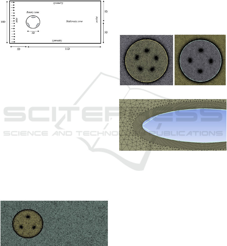
2.3 Boundary Conditions
The dimension of domain boundary in this study is
determined namely 10D x 20D (Fig. 3). The length
and width of domain boundary 20D and 10D
respectively were studied and recommended by
Marsh et al (2015). The domain boundary consists of
two main zones, namely, rotary, and stationary for
using the meshing method. The position of the
circular turbine is on the 5D from the inlet, 15D from
the outlet, and in the middle of the symmetry wall.
ISOCEEN 2019 - The 7th International Seminar on Ocean and Coastal Engineering, Environmental and Natural Disaster Management
48
The boundary conditions are simulated in the 2D
CFD model with the use of free stream conditions. In
this study case, the turbine without use arms and
shaft. The inlet and outlet conditions are set in the
velocity of 1.5 m/s and pressure 0 Pa, respectively.
The walls are set as symmetry so that the fluid has the
same distributions at the top and bottom of the walls.
Figure 3: Domain boundary of the turbine model.
2.4 Meshing
The meshing is part of designing CFD simulations, a
net strategy which is a process that determines the
final results of design studies using CFD. The use,
the number of elements in the meshing that is more
and finer will produce a better the final results, and
vice versa. However, the number of elements that
are many and smooth requires a long time. So, it
takes a meshing strategy with smooth elements and
not at the same time. In this study, the statistics of
meshing elements are used 16,090, 167,020, and
174,375 at the blades 3, 4, and 5, respectively. The
number of elements based on the criteria for grid
independence a study was conducted by Marsh et al
(2017).
In this study, the structure of meshing uses the
triangle method. The process of meshing structure in
the 2D CFD model is arranged so that the rotary
zone is made denser than the stationary zone and the
blade zone is made denser than the rotary zone. The
results of the meshing structure in this study can be
shown in Fig. 4.
Figure 4: Meshing of domain boundary the basic turbine.
The mesh density is refined (Fig. 5) in the area of
the blades, interior fluids, and interface zone by
specifying the relevance center, smoothing, span
angle center, face sizing, and edge sizing to receive
hydrodynamic flow (Marsh et al., 2015). Edge sizing
in all areas the turbine blades are the same at 0.0004
m. And then face sizing in the area of the turbine
and the interior fluids are set at 0.05 m and 0.054,
respectively.
The Inflation layers are utilized to control cell
heights near all the turbine blades wall to resolve the
boundary layer flow (Marsh et al., 2015), shown in
Fig. 6. According to recent studies, the inflation
layer set at 20 layers and the global growth rate set
at 1.2 (Satrio et al., 2018).
Figure 5: Refinement meshing of the variations turbine.
Figure 6: Inflation layers of the blade.
2.5 Solver Setup
In this study uses 6 core internal parallel processing
for simulation the turbine blades with 2D CFD. The
code is used to solved incompressible turbulence of
Unsteady Reynolds Averaged Navier Stokes (U-
RANS) equations. The k-ω SST turbulence model is
utilized because it has a good accuracy model both
free stream and boundary layer region (Marsh et al.,
2016). Beside that often is used by researchers for
vertical axis current turbines
(Dai and Lam, 2009;
Castelli et al., 2010; S Lain, 2010; Malipeddi and
Chatterjee, 2012; Marsh et al, 2012, 2013 and 2014).
The setting of the solution method at pressure
velocity uses Semi-Implicit Method for Pressure
Linked Equation (SIMPLE) for algorithm scheme
and overall is set as second-order.
Variation Number of Blades for Performance Enhancement for Vertical Axis Current Turbine in Low Water Velocity in Indonesia
49
In this research simulation generally uses general
transient type settings for an application to water
fluid types. General transient type settings for an
application to water fluid types. So that in the
material setting choose the type of fluid that is water
with a density of 998.2 kg/m
3
. Furthermore, at the
cell zone condition step, to input the rotational speed
at TSR 1.5, 2, and 2.5 are 4.92 rad/s, 6.56 rad/s, and
8.21 rad/s, respectively. The current speed data is set
at the boundary condition-stage of 1.5 m/s.
After that, residual monitor for convergence is
set at overall equation 10
-4
and the maximum of
iteration is 70. The input of calculation simulation is
the number of time step (NTS) and time step size
(TSS). In this study uses increment angle 0,9 degree
and 6 rotation of turbine at all TSR. TSS represents
the addition of angles each time the turbine rotates
and NTS represents how many turbines rotated
during the simulation (Satrio et al., 2018).
3 RESULTS AND DISCUSSION
3.1 Verification of 2D CFD Model
Verification this study of 2D CFD model simulation
is carried out against was published data of the 3D
CFD model by Marsh et al (2015). This study case
compares the basic turbine 2D CFD with the 3D
CFD model, shown in Fig. 7. The curve of Cp-TSR
shows that the result of simulation 2D CFD has a
similar trend with simulation 3D CFD. The result of
Cp in this study shows that at TSR 1.5 represents
low water velocity, different 16% with the 3D CFD
model data. Differences in the value of Cp due to the
use of different model dimensions and this study
without uses of arm and shaft model design.
Generally, at the 2D CFD model turbine by
researchers without use arm and shaft.
Figure 7: Verification 2D CFD result with the published
3D CFD data.
3.2 Effect of Blade Number on Torque
The first performance parameter in this study case is
about the torque of the turbine. Output simulation
with the 2D CFD model is data of torque coefficient
(Ct) to represent the torque of the turbine. The curve
of Ct-TSR in Fig. 8, shows the value of Ct and TSR
at the basic turbine (blade 3) and the variations
turbine (blades 4 and 5).
The value of Ct will determine the value of
torque by using equation 2. The value of the torque
at all the turbine blades is shown in Table 2.
Figure 8: Ct-TSR curve at all the turbine blades.
Table 2: The value of torque (N.m).
TSR T 3 blade T 4 blade T 5 blade
1.5 9.353 19.925 17.983
2 23.996 33.185 31.330
2.5 27.278 33.229 31.352
Based on Fig. 8 and Table 2 show that at all
TSR, the blades 4 are higher torque than the blades 3
and 5. This study uses at TSR below 3 because it
represents low water velocity. This study shows that
at all low TSR ranges the blades 4 have the best
performance with torque parameters. The torque of
the blades 4 is increased by 21.8% from the blades
3, whereas the blades 5 is increased by 15% from the
blades 3 or is decreased by 5.6% from the blades 4.
So, this study shows that performance enhancement
in the low water velocity is obtained by the turbine
blades 4, with torque parameters.
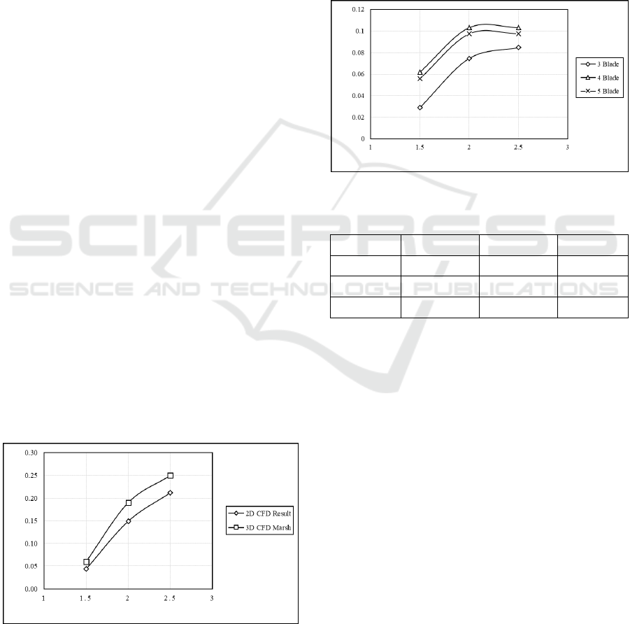
3.3 Effect of Blade Number on Solidity
The second performance parameter in this study case
is about the solidity of the turbine. The value of
turbine solidity is obtained by using equation 1. The
more the number of blades, the greater the value of
turbine solidity (σ) is shown in Table 3.
TSR
Cp
TSR
Ct
ISOCEEN 2019 - The 7th International Seminar on Ocean and Coastal Engineering, Environmental and Natural Disaster Management
50
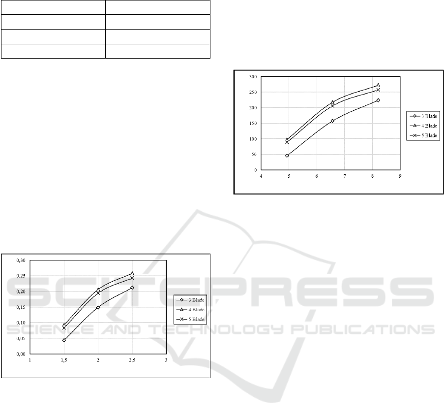
Table 3: The value of solidity.
The number of blades (N) The value of solidity (σ)
3 0.07
4 0.09
5 0.11
Based on Table 3 show that the turbine blades 3,
4, and 5 have the value of solidity 0.07, 0.09, and
0.11, respectively. The effect of solidity on the
turbine performance can be shown through a curve
Cp-TSR, in Fig. 9. The power coefficient increase
with the increase in turbine solidity from the turbine
blades 3 (σ = 0.07). However, at the turbine solidity,
0.11 represents the turbine blades 5 decreases from
blades 4. The authors predict that this is due to a
loose lift force because of the turbine more solid.
The highest Cp occurs at TSR 2.5 on blades 4 with a
value of 0.26. However, the solidity 0.09 represents
the turbine blades 4 improve performance to 21.8%.
So, this study shows that performance enhancement
in the low water velocity is obtained by the turbine
blades 4, with solidity parameters (σ = 0.09).
Figure 9: Cp-TSR curve at all the turbine blades.
3.4 Effect of Blade Number on Power
The third performance parameter in this study case
is about the power of the turbine. The value of
power is determined by the rotational speed (ω) in
rad/s using equation 4. The curve of P-ω in Figure 9
shows the effect of blade number on power (P) with
the input of rotational speed namely, 4.92 rad/s, 6.56
rad/s, and 8.21 rad/s.
Based on Fig. 10 shows that the power of the
turbine is influenced by rotational speed according
to equation 4. The correlation between power output
and rotational speed are comparable. The higher the
rotational speed is the higher the power in watt at all
blade numbers. The highest power occurs at TSR 2.5
on blades 4 with a value of 273 watts. The power of
the blades 4 is increased by 21.8% from the blades
3, whereas the blades 5 is increased by 15% from the
blades 3 or is decreased by 5.6% from the blades 4.
However, the value of power at the turbine blades 4
to improve performance to 21.8% from blades 3. So,
this study case shows that performance enhancement
in the low water velocity is obtained by the turbine
blades 4, with power parameters.
Figure 10: The results of the turbine power.
4 CONCLUSIONS
The simulation of variation of the number of blades
3, 4, and 5 successfully is done. The final results of
this study case show that the number of blades can
improve the performance of the turbine model on all
low TSR ranges. The blades 4 and 5 are increased by
21.8% and 15% respectively from the blades 3 on
the TSR 2.5. The highest performance is obtained by
the number of blades 4 on TSR 2.5 with the value of
Cp 0.26. So, this study case will choose the blades 4
for further research with the experimental method.
ACKNOWLEDGEMENTS
This research is done with the assistance of several
parties. Authors thanks to the team research and
appreciation to the directorate general of resources
for science, technology, and higher education; the
ministry of research, technology, and education; the
Republic of Indonesia, which fund this research on
the scheme called, “The Thesis Magister Research”
under decree number 6/E/KPT/2019 on 02/19/19,
and contract number 5/E1/KP.PTNBH/2019 and
778/PKS/ITS/2019 on 03/29/19, and on the scheme
called, “The Basic Research” under decree number
6/E/KPT/2019 on 02/19/19, and contract number
5/E1/KP.PTNBH/2019 and 847/PKS/ITS/2019 on
03/29/19.
TSR
ω
Cp
Pt
Variation Number of Blades for Performance Enhancement for Vertical Axis Current Turbine in Low Water Velocity in Indonesia
51

REFERENCES
Bachant, P. and Wosnik, M. (2015). Performance
measurements of cylindrical- and spherical- helical
crossflow marine hydrokinetic turbines, with estimates
of exergy efficiency. Renew Energy.
Castelli, M.R., G. Ardizzon, L. Battisti, E. Benini, G.
Pavesi. (2010). Modeling strategy and numerical
validation for a Darrieus vertical axis micro-wind
turbine. in: ASME 2010 International Mechanical
Engineering Congress and Exposition, Vancouver,
British Columbia, Canada.
Dai YM, W. Lam. (2009). Numerical study of straight-
bladed darrieus-type tidal turbine. Proc. Institution
Civ. Eng. Energy.
Duvoy, P., Hydrokal., T. H. (2012). A Moduleforin-stream
Hydro Kinetic Resource Assessment. Computer &
Geosciences. 39: 171–81.
Fish, F. E., and Battle, J. M. (1995). Hydrodynamic
Design of the Humpback Whale Flipper. Journal of
Morphology,pp.5160.doi:10.1002/jmor.1052250105.
Vol. 225
H. Johari, C. Henoch, D. Custodio, and A. Levshin.
(2007). Effects of Leading-Edge Protuberances on
Airfoil Performance, AIAA Journal Vol. 45, No. 11.
Hydrovolts. (2006). In-stream Hydrokinetic Turbines.
Power tech Labs, Available from hydrovolts.com.
Jing, Fengmei. (2014). Experimental Research on Tidal
Current Vertical Axis Turbine with Variable-Pitch
Blades. Ocean Engineering, 88:228-241.
Khan, M. J., Bhuyan, G., Iqbal, M. T., Quaicoe, J. E.
(2009). Hydro kinetic Energy Conversion Systems and
Assessment of Horizontal and Vertical Axis Turbines
for River and Tidal Applications: A Technology Status
Review. Applied Energy. 86(10): 1823–35.
Kirke, B. K. and Lazauskas, L. (2011). Limitations of fixed
pitch Darrieus hydrokinetic turbines and the challenge
of variable pitch. Renewable Energy 36 2011 893-
897: Elsevier.
Li, Shengmao dan Yan Li. (2010). Numerical study on the
performance effect of solidity on the straight-bladed
vertical axis wind turbine. Scientific Research Fund of
Heilongjiang Provincial Education Department
(No.:1153h01); Scientific Research Foundation for the
Returned Overseas Chinese Scholars.
Madi, M E N Sasono, Y S Hadiwidodo and S H Sujiatanti.
(2019). Application of Savonius Turbine behind The
Propeller as Energy Source of Fishing Vessel in
Indonesia. IOP Conf. Series: Materials Science and
Engineering, IOP Publisher.
Malipeddi A.R. and D. Chatterjee. (2012). Influence of
duct geometry on the performance of Darrieus
hydroturbine. Renew. Energy.
Marsh, D. Ranmuthugala, I. Penesis, G. Thomas. (2012).
Three dimensional numerical simulations of a
straight-bladed vertical axis tidal turbine. in:
Proceedings of the 18th Australasian Fluid Mechanics
Conference, Launceston, Tasmania.
Marsh, D. Ranmuthugala, I. Penesis, G. Thomas. (2013).
Performance predictions of a straight-bladed vertical
axis turbine using double-multiple streamtube and
computational fluid dynamics. J. Ocean Technol.
Marsh, D. Ranmuthugala, I. Penesis, G. Thomas. (2014).
Numerical simulation of straight-bladed vertical axis
turbines, in: 2nd Asian Wave and Tidal Energy
Conference (AWTEC), Tokyo Japan.
Marsh, D. Ranmuthulaga, I. Penesis and G. Thomas.
(2015). Three dimensional numerical simulation of
straight-bladed vertical axis tidal turbines
investigating power output, torque ripple and
mounting force, Renewable Energy 83 67-77: Elsevier.
Marsh, D. Ranmuthulaga, I. Penesis and G. Thomas.
(2015). Numerical investigation of the influence of
blade helicity on the performance characteristic of
vertical axis tidal turbine, Renewable Energy 81 926-
935: Elsevier.
Marsh, D. Ranmuthulaga, I. Penesis and G. Thomas.
(2016). Numerical simulation of the loading
characteristics of straight and helical-bladed vertical
axis tidal turbines. Renewable Energy 94 418-428:
Elsevier.
Marsh, D. Ranmuthulaga, I. Penesis and G. Thomas.
(2017). The influence of turbulence model and two and
three-dimensional domain selection on the simulated
performance characteristics of vertical axis tidal
turbines, Renewable Energy 105 106-116: Elsevier.
Mukhtasor, Susilohadi, Erwandi, Pandoe, W., Iswadi, A.,
Firdaus, A. M., Prabowo, H., Sudjono, E., Prasetyo, E.
dan Iluhade, D. (2014). Potensi Energi Laut
Indonesia. Badan Litbang Kementrian Energi dan
Sumberdaya Mineral (ESDM) dan Asosiasi Energi
Laut Indonesia (ASELI).
Quang Le, Kwang Soo Le, Jin Soon Park and Jin Hwan
Ko. (2014). Flow-driven rotor simulation of vertical
axis tidal turbines: A comparison of helical and
straight blades. Int. J. Nav. Archit. Ocean Eng.
Rawlings G. (2008). Parametric characterization of an
experimental vertical axis hydro turbine. MSC
dissertation. University of British Columbia.
Satrio, Dendy., I.K.A.P Utama., Mukhtasor. (2016).
Vertical Axis Current Turbine Advantages and
Challenges Review. Proceeding of Ocean, Mechanical
and Aeroscope. Science and Engineering Vol.3, Hal.
64-71. Universiti Malaysia Terengganu, Malaysia.
Satrio, Dendy., I.K.A.P Utama., Mukhtasor. (2018). The
influence of time step setting on the CFD simulation
result of vertical axis tidal current turbine. Journal of
Mechanical Engineering and Sciences. Volume 12,
Issue 1, Hal. 3399-3409. UMP Publisher.
Satrio, Dendy., I.K.A.P Utama., Mukhtasor. (2018).
Numerical Investigation of Contra Rotating Vertical-
Axis Tidal Current Turbine. Journal of Marine Science
and Application. Hal. 3399-3409. UMP Publisher.
Satrio, Dendy., I.K.A.P Utama., Mukhtasor. (2018).
Performance Enhancement Effort for Vertical Axis
Current Turbine in Low Water Velocity.
Proceeding of The 4
th
Asian Wave and Tidal Energy
Converence (AWTEC). National Taiwan Ocean
University, Taiwan.
ISOCEEN 2019 - The 7th International Seminar on Ocean and Coastal Engineering, Environmental and Natural Disaster Management
52

S. Lain. (2010). Simulation and evaluation of a straight-
bladed darrieus-type cross flow marine turbine. J. Sci.
Industrial Res.
Winchester, J.D. dan Quayle S.D. (2009). Torque ripple
and variable blade force: A comparison of Darrieus
and Gorlov-type turbines for tidal stream energy
conversion. Proceedings of the 8th European Wave
and Tidal Energy Conference, Uppsala, Sweden.
Zeiner-Gundersen, D. H. (2015). A novel flexible foil
vertical axis turbine for river, ocean, and tidal
applications. Applied Energy 151 2015 60–66:
Elsevier.
Variation Number of Blades for Performance Enhancement for Vertical Axis Current Turbine in Low Water Velocity in Indonesia
53
