
Analysis of the Effect of Gross Domestic Product and Price of Food
Commodities on Inflation in Indonesia
Kurnia Novianty Putri
1
, Fitrawaty
2
and Sri Fajar Ayu
3
1
Department of Economy Post Graduate School, State University of Medan, North Sumatera
2
Department of Economy, State University of Medan, North Sumatera
3
Department of Economy, State University of North Sumatera, North Sumatera
Keywords: Gross Domestic Product, Price of Food Commodities, Inflation, Error Correction Model
Abstract: The purpose of this study was to find out how the effect of gross domestic product, the price of rice, the
price of bulk cooking oil, the price of sugar, the price of curly red chili, and the price of chicken meat on
inflation in Indonesia. The research method used was the regression technique with Error Correction Model
data analysis. Data was processed using E-views 7.0. At unit root test, it is known that all observation
variables were stationary. In determining the optimal lag length shows the criteria of Akaike Information
Criterion (AIC), Schwarz Criterion (SC) and Human Quinn Criterion (HQ) and the smallest value was
chosen between the optimal lag value of Schwarz Criterion (SC) at lag 1. The cointegration test results
indicate that the variable was in a long-term equilibrium condition, so the regression results were
cointegrated regression. Result of the classic assumption test were, data was normally distributed, free from
autocorrelation, liberaly from the symptoms of multicollinearity, and free from the heteroscedasticity. The
results obtained were the effect of gross domestic product variables, price of medium quality rice, price of
bulk cooking oil prices in the short term positif and significant on inflation in Indonesia. Price of curly red
chilli in the short term positif and not significant on inflation in Indonesia. Price of sugar and price of
chicken meat in the short term negatif and not significant on inflation oi Indonesia. Also found that the
effect of gross domestic product variables in the long term positif and significant on inflation in Indonesia,
price of medium quality rice and price of curly red chilli in the long term positif and not signifikan on
inflation in Indonesia. Price of bulk cooking oil prices, price of sugar, and price of chicken meat in the long
term all not significant on inflation of Indonesia.
1 INTRODUCTION
Inflation is an increase in the prices of goods
continuously in a certain period. The high inflation
rate would reduce economic growth. The term of
economic growth was used to describe the progress
of economic development in a country. A country is
said to experience growth, if the product of its goods
and services increased or in other words there is a
development of a country's potential Gross Domestic
Product (GDP).
The increase in GDP have a good and bad effect
on Indonesia's economic condition. One of them is
the increase in GDP which is the cause of demand-
side inflation, the consumptive behavior of the
Indonesian people causes demand to increase so that
prices can increase. In 2008 the value of GDP was
only Rp. 1,524,123,000,000,000.00. Then in 2015 it
grew to Rp. 2,272,929,000,000,000.00 despite the
increase in GDP value good for Indonesia's
economic growth, but could cause inflation. In
Nugroho's research (2012) states that GDP has a
positive impact on inflation.
In essence, community welfare will be achieved
well if the basic needs of the community can be
realized. One of the basic human needs is food.
Therefore, the fulfillment of a country's food needs
is an absolute matter. Based on the Food Price Index
of the Food and Agriculture Organization (FAO),
world food commodity prices have continued to
increase since 2000. The world food crisis that
occurred between 2007-2008 was marked by the
price of food commodities which rose sharply and
then reached its highest point in 2011-2012. Food
Price Index data showed that the level of world food
prices in 2011 was the latest record for the past ten
years (published by the World Bank). The
economies of countries in the world, especially
developing countries with the largest expenditure of
Putri, K., Fitrawaty, . and Ayu, S.
Analysis of the Effect of Gross Domestic Product and Price of Food Commodities on Inflation in Indonesia.
DOI: 10.5220/0009502404730480
In Proceedings of the 1st Unimed International Conference on Economics Education and Social Science (UNICEES 2018), pages 473-480
ISBN: 978-989-758-432-9
Copyright
c
2020 by SCITEPRESS – Science and Technology Publications, Lda. All rights reserved
473
households, are food expenditure that has an impact
and influence on the economy of the country.
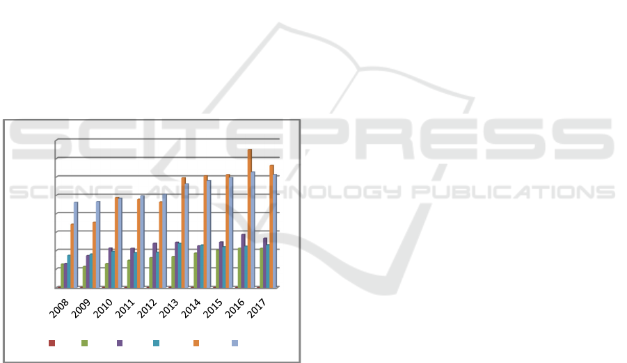
The results of empirical research showed that
food commodity prices is one of the biggest factors
affecting the high inflation rate in developing
countries such as China, India and Indonesia (Lee &
Park, 2013). Data from FAO showed that the
average inflation of Indonesian food commodities in
the past ten years was 10.36%, while Thailand was
around 5.57%, followed by Malaysia and the
Philippines around 2.8%. Empirical studies show
that the poor at both the national and regional levels
are very sensitive and vulnerable to being affected
by rising food inflation in recent years (Pratikto &
Ikhsan, 2015). Food inflation is a significant
contributor to inflation in Indonesia. Fluctuations in
food commodity prices had become an important
problem in controlling inflation in Indonesia. High
inflation will cause people's real income to decline
so that people's purchasing power decreases. Furlog
in Astari (2015) stated that fluctuations in food
commodity prices can be used as an inflation
indicator because it has the ability to respond
quickly to various economic shocks that occur, such
as increasing supply and demand shocks.
Figure 1: Food Commodity Price Development from
2008 up to 2017 (In Rupiah)
Based on the description previously stated, it is
considered important to conduct research on how
much effect the fluctuations in food commodity
prices and gross domestic product have on inflation
in Indonesia.
2 RESEARCH METHOD
The scope of the observations made in this study are;
inflation data, Gross Domestic Product (GDP), and
food commodity price data, namely medium quality
rice price data, bulk cooking oil prices, local sugar
prices, curly red chili prices, chicken meat prices in
Indonesia using time series data in the period of
2008: Q1 - 2017: Q4. This research was limited by
time series secondary data in the form of annual
reports that have been compiled and have been
published by related parties namely Bank Indonesia
(BI), Central Statistics Agency (BPS), Logistics
Agency (Bulog), and Development Planning Agency
(BAPPENAS). Data is also obtained from books and
other research results related to the research
conducted.The increase in GDP have a good and bad
effect on Indonesia's economic condition. One of
them is the increase in GDP which is the cause of
demand-side inflation, the consumptive behavior of
the Indonesian people causes demand to increase so
that prices can increase. In 2008 the value of GDP
was only Rp. 1,524,123,000,000,000.00. Then in
2015 it grew to Rp. 2,272,929,000,000,000.00
despite the increase in GDP value good for
Indonesia's economic growth, but could cause
inflation. In Nugroho's research (2012) states that
GDP has a positive impact on inflation.
Data analysis used Error Correction Model,
which is a form of model used to determine the
effect of short-term and long-term independent
variables on the dependent variable. In addition to
knowing the effect of economic models in the short
and long term, the ECM model can also overcome
data that is not stationary characterized by the
presence of high R2 but has a low Durbin Watson
value (Shocrul, 20011: 137). Data analysis in this
study utilized Microsoft Excel 2007 software and
then processed by E-Views 7.0. The model used in
this study show below.
IINF
t
= f (PDB
t
, BER
t
, MGC
t
, GUL
t
, CMK
t
, DAY
t
)
………………..…… (1)
IINF
t
= β
0
+β
1
PDB
t
+ β
2
BER
t
+ β
3
MGC
t
+ β
4
GUL
t
+
β
5
CMK
t
+ β
6
DAY
t
+εi
Where :
INF = rate of Inflation (%)
PDB = Produk Domestik Bruto (Milyar Rupiah)
BER = Medium quality rice prices (Rupiah)
MGC = Bulk cooking oil prices (Rupiah)
GUL = Local sugar prices (Rupiah)
CMK = Curly red chili prices (Rupiah)
DAY = Chicken meat prices (Rupiah)
β
0
= Constant
0
5000
10000
15000
20000
25000
30000
35000
40000
INF BER GUL MGC CMK DAY
UNICEES 2018 - Unimed International Conference on Economics Education and Social Science
474
β
1
: β
2
: β
3
: β
4
: β
5
= Coefficient of Regression
εi = Disturbance error
3 RESULTS AND DISCUSSION
Data of inflation rates in Indonesia from 2008 to
2017, data of Indonesia's Gross Domestic Product
(GDP) growth, data of changes in medium quality
rice prices in Indonesia, data of changes in bulk
cooking oil prices in Indonesia, data of changes in
sugar prices in Indonesia, data of changes Curly red
chili prices in Indonesia, and data of changes in
prices of chicken meat in Indonesia are presented
respectively in Figure 2, Figure 3, Figure 4, Figure
5, Figure 6, Figure 7, and Figure 8.
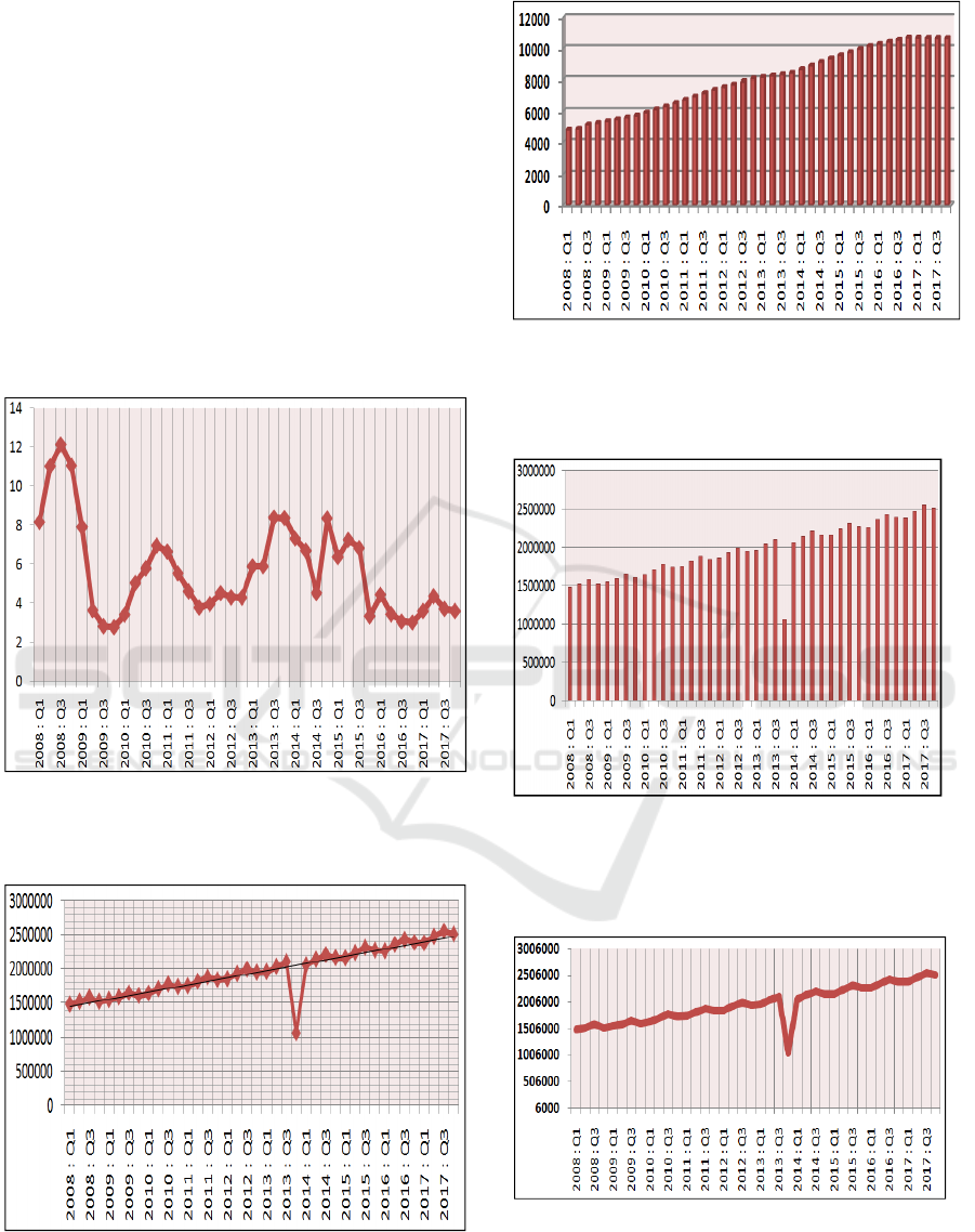
Source : processed form Cenral Statistic Agency
Figure 2: Presentation of Graphs of Inflation Rate in
Indonesia from 2008:1 to 2017:4
Source : processed form Cenral Statistic Agency
Figure 3: Graph of Gross Domestic Product Growth
in Indonesia Years from 2008: 1 to 2017: 4
Source : processed form Cenral Statistic Agency
Figure 4: Graph of change of Medium Quality Rice
Prices in Indonesia from 2008: 1 to 2017: 4 (In
Rupiah Currency)
Source : processed form Cenral Statistic Agency
Figure 5: Graph of Changes in Bulk Cooking Oil
Prices in Indonesia from 2008: 1 to 2017: 4 (In
Rupiah currency)
Source : processed form Cenral Statistic Agency
Figure 6: Graph of Changes in Local Sand Sugar
Prices in Indonesia from 2008: 1 to 2017: 4 (In
Rupiah currency)
Analysis of the Effect of Gross Domestic Product and Price of Food Commodities on Inflation in Indonesia
475
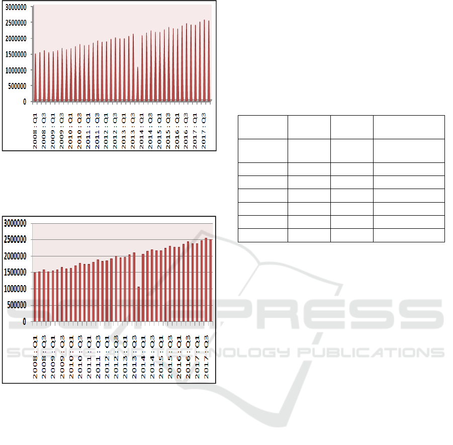
Source : processed form Cenral Statistic Agency
Figure 7: Graph of Changes in Curly Red Chilli
Prices in Indonesia from 2008: 1 to 2017: 4 (In
Rupiah currency)
Figure 8: Chart of Chicken Meat Prices in Indonesia
from 2008: 1 to 2017: 4 (In Rupiah currency)
Stationarity Test (Unit Root Test)
Stationary data is data that shows the mean, variance
and autovariance (in lag variations) remain the same
at any time when the data is formed or used,
meaning that with stationary data the time series
model can be said to be more stable. The data
stationarity test used in this study is the Phillips
Perron Test (PP test) with no trend constants is a test
developed by Philips and Perron which aims to
determine data stationarity at the level. If the results
of the unit data root tests are obtained partially or all
data is not stationary, it is necessary to proceed to
the degree of integration test. Variables used in this
study were none stationary with a probability level
of α = 5% at the level of the level. Therefore it is
necessary to carry out further tests by using an
integration degree test (different) to find out at what
degree the data will be stationary. Based on the
calculation results obtained values at the first
different level are also not all stationary data. Then
stationary test observations were carried out again at
the second different level. Based on the calculation
results obtained the calculated value for all
stationary variables at the level of second different.
Tabel 1: Unit Root Test Results with the ADF
Method in Second Different
Variables Value of
Statistic
Proba
bility
Interprettatio
n
LNINF -
6.0669
0.0000 Stationer
LNPDB -6.2819 0.0000
Statione
r
LNBER -14.828 0.0000
Statione
r
LNMGC -5.9389 0.0000
Statione
r
LNGUL -4.4753 0.0013
Statione
r
LNCMK -6.5923 0.0000
Statione
r
LNDAY -6.1009 0.0000
Statione
r
From Table 1 it was found that all calculated
ADF values showed that all stationary observation
variables were in second different after being
reduced twice. After it is believed that all
observation variables have the same degree of
integration, cointegration tests can be performed on
the observation variables
Determination of Optimal Lag Length
Lag Length Test (Determination of Optimal Lag)
Optimal lag is the number of lags that have a
significant influence or response. Determination of
Lag According to Alfian (2011) besides influencing
himself, a variable can also influence other
variables. The lag testing used in this study uses the
Akaike Information Criterion (AIC) approach,
Schwarz Information Criterion (SC) and Hannan
Quinn (HQ). The results show the Akaike
Information Criterion (AIC), Schwarz Criterion (SC)
and Human Quinn Criterion (HQ) criteria and the
smallest value is chosen between the optimal lag
Schwarz Criterion (SC) value in lag 1.
Cointegration Test.
Cointegration tests can be expressed as a test of the
balance relationship or long-term relationship
between economic variables as desired in the theory
of econometrics (Insukindro, 1999). The method
used for the cointegration test in this study is the
Engle-Granger Cointegration Test method. The
Agumented Dickey Fuller (ADF) test results can be
seen in Table 2.
UNICEES 2018 - Unimed International Conference on Economics Education and Social Science
476

Tabel 2: Results of Cointegration Test
V
ariable critical value of
ADF
ADF
Prob
abi-
lity
ECT
1% 5% 10%
-3.6329 -2.9484 -2.6128 -4.922 0.000
3
Table 2 shows the ADF test value> Critical
Value which is -4,922, then indicates cointegration
between regression variables between gross
domestic product value, medium quality rice price,
bulk cooking oil price, local sugar price, curly red
chili price, price of chicken meat to inflation. This
indicates that the variable is said to be in a long-term
equilibrium condition, so the regression results are
cointegrated regression.
Error Correction Domowitz-El Badawi Model
The ECM model developed by Domowitz and El
Badawi is based on the fact that the economy is in a
state of imbalance. According to this model, the
ECM model is valid if the error correction
coefficient sign is positive and statistically
significant. This error correction coefficient value is
located 0 <g <1 (Widarjono, 2009: 336). Following
the approach developed by Domowitz and El
Badawi, the raw form of ECM was obtained as
follows:
To find out the specification of the model with
ECM is a valid model, it can be seen in the results of
statistical tests on the coefficient of ECT. To obtain
the magnitude of the standard deviation of the long-
term regression coefficient in the ECT model
estimation.
Error Correction Model can explain the behavior
of short-term and long-term influence on
independent variables on the dependent variable.
The processing estimation results are carried out
using the Eviews 7 program, with the ECM linear
regression model, the results of data processing are
shown at Table 3.
Tabel 3: Results of Regression Estimation with Error
Correction Domowitz-El Badawi model
V
ariabl
e
Coefisie
n
Statistic - t
P
robability
A
djust
ed R
2
C 8.5110 0.4982 0.6229
0.73
34
Short term
D
(LNPDB) 0.3198 2.6485 0.0381
D
(LNBER) 19.2491 2.6940 0.0127
D
(LNMGC) 12.67267 2.9262 0.0074
D
(LNGUL) -2.6495 -0.9734 0.3400
D
(LNCMK) 2.0487 0.9981 0.3282
D
(LNDAY) -14.9658 -2.0463 0.0518
Long term
L
NPDB(-1) 0.0300 2.806059 0.0309
L
NBER(-1) 1.4953 1.2781 0.2134
L
NMGC(-1) -1.5671 -1.2668 0.2174
L
NGUL(-1) -0.9443 -0.6893 0.4972
L
NCMK(-1) 0.8277 0.7575 0.4561
L
NDAY(-1) -0.4710 -0.2771 0.7841
E
CT 0.4943 5.8954 0.0000
The results of the Domowitz-El badawi error
correction model obtained a positive and significant
coefficient value (probability value < absolute price
of critical value for α = 5%). this indicates that the
ECM model used in this study is valid or
appropriate. in this study the value of ect (error
correction term) is 0.4943 with a t-statistic value of
5.8954 > t-table 5% df 40 = 1.6838 significant at α =
5%. the ECT coefficient value is positive and
statistically significant means that the Domowitz-El
Badawi ECM specification model used in this study
is valid (Widarjono, 2009).
Classical Assumption Test
Normality Test. The normality test is used to test
whether in the regression model, the independent
variable and the dependent variable are normally
distributed or not. This test was carried out with
Jarque Bera. The assumption of normality can be
fulfilled the value of the Sig value > 0.05%. Based
on data processing, the J-B statistical probability
value is 0.2693 > α = 5% (0.05). So, it can be
concluded that the data used in the ECM model is
normally distributed.
Autocorrelation Test. The result of autocorrelation is
that the estimated parameters are biased and the
variants are minimum, so they are not efficient
Analysis of the Effect of Gross Domestic Product and Price of Food Commodities on Inflation in Indonesia
477

(Damodar Gujarati, 2004). To test the presence or
absence of autocorrelation, one of them is known by
conducting the Breusch-Godfrey Test or the
Langrange Multiplier (LM) Test. From the results of
the LM test if the value of the Prob. F count is
greater than alpha level 0.05 (5%) stating that the
model is free from autocorrelation. Criteria for
rejection or acceptance can be made using the
Durbin-Watson Table. The criteria for acceptance or
rejection to be made with the values of dL and dU
are determined based on the number of independent
variables in the regression model (k) and the number
of samples (n). The values of dL and dU can be seen
in Table DW with a significance level (error) of 5%
(α = 0.05). Number of independent variables: k = 6.
Number of samples: n = 40. Table Durbin-Watson
shows that the value of dL = 1.1754 and the value of
dU = 1.8538 so that the criteria for whether or not
autocorrelation can be determined. Durbin-Watson
(DW) value is 2.0833, this value is greater than
1.8538 and smaller than 2.4922 so it can be
concluded that the ECM model is free from the
problem of autocorrelation.
Multicollinearity Test. Multicollinearity is the
condition of a linear relationship between
independent variables (Wing Wahyu, 2009). A good
regression model should not have a correlation
between independent variables. If the independent
variables correlate with each other, then these
variables are not orthogonal (Imam Ghozali, 2006).
Orthogonal variables are independent variables with
the value of correlation between each independent
variable equal to zero. Multicolinerity in this study
was tested using the partial correlation method
between independent variables. The rule of tumb
from this method is if the correlation coefficient is
high enough above 0.85, we expect there is
multicollinearity in the model (Widarjono, 2009:
106). The multicollinearity test results show that all
independent variables have a correlation coefficient
value below 0.85 so that it can be concluded that the
ECM model is free from the symptoms of
multicollinearity.
Heteroscedasticity Test. Heteroscedasticity aims to
test whether in the regression model there is an
inequality of variance from the residual one another
observation. A good regression model is
homoschedasticity or heteroscedasticity does not
occur. To test for the presence or absence of
heteroscedasticity Glejser Test can be used. If the
value is Prob. F count is greater than alpha level
0.05 (5%) then Ho is accepted which means there is
no heteroscedasticity. A good regression model is a
regression that does not occur heteroscedasticity. If
the significance value is > 0.05 then
homoskedasticity occurs and if the significance
value is <0.05, heteroscedasticity occurs.
Hypothesis Test
t-test. The t-statistical test is used to determine the
effect of each independent variable on the dependent
variable (Ghozali, 2013). Determine the acceptance
criteria or rejection of H0, namely by looking at
significant values. If p-value is < 0.05, then Ho is
rejected or Ha is accepted and if p-value is > 0.05
then Ho is accepted or Ha is rejected. The F-Statistic
Test is used to find out whether the independent
variables simultaneously or simultaneously affect
the dependent variable.
In the short term t-statistics and the probability of
each variable gross domestic product (GDP) t-
statistic = 2.6485 and the coefficient value = 0.0319
(prob = 0.0381) shows that the variable gross
domestic product (GDP) has a positive effect and
significantly influences inflation in Indonesia.
Medium quality rice price variable (BER) with t-
statistic value = 2.6940 and coefficient value =
19.249 (prob = 0.0127) shows that medium quality
rice (BER) variable has a positive influence and
significantly influences inflation in Indonesia. The
variable price of bulk cooking oil (MGC) with a
value of t-statistic = 2.9262 and the coefficient value
= 12.6726 (prob = 0.0074) shows that the variable
bulk cooking oil (MGC) has a positive and
significant effect on inflation in Indonesia. Variable
sugar (GUL) with t-statistic value = -0.9734 and
coefficient value = -2.6495 (prob = 0.3400) shows
that the variable price of sugar (GUL) has a negative
effect and does not significantly influence inflation
in Indonesia. Red curly chili variable (CMK) with t-
statistic value = 0.9981 and coefficient value 2.0487
(prob = 0.3282) shows that the red curly chili
variable (CMK) has a positive effect and does not
significantly influence inflation in Indonesia.
Chicken meat variable (DAY) with t-statistic value =
-2.0463 with coefficient value = -14.9658 (prob =
0.0518) shows that the variable price of chicken
meat has a negative effect and does not significantly
influence inflation in Indonesia.
In the long term the gross domestic product (GDP)
variable t-statistic = 2.8060 and the coefficient value
= 0.0300 (prob = 0.0309) shows that the variable
gross domestic product (GDP) is positively
influential and significantly influences inflation in
Indonesia. Medium quality rice price variable (BER)
with t-statistic value = 1.2781 and coefficient value
= 1.4953 (prob = 0.2134) shows that the medium
UNICEES 2018 - Unimed International Conference on Economics Education and Social Science
478

quality rice (BER) variable has a positive effect and
does not significantly affect inflation in Indonesia.
Variable price of bulk cooking oil (MGC) with t-
statistics value = -1.2668 and coefficient value = -
1.5671 (prob = 0.2174) shows that the variable bulk
cooking oil (MGC) has a negative effect and does
not significantly affect inflation in Indonesia.
Variable sugar (GUL) with t-statistic value = -.6893
and coefficient value = -0.9443 (prob = 0.4972)
shows that the variable price of sugar (GUL) has a
negative effect and does not significantly influence
inflation in Indonesia. Red curly chili variable
(CMK) with t-statistic value = 0.7575 and
coefficient value 0.8276 (prob = 0.4561) shows that
the curly red chili variable (CMK) has a positive
effect and does not significantly influence inflation
in Indonesia. Chicken meat variable (DAY) with t-
statistic value = -0.2771 with coefficient value = -
0.4710 (prob = 0.7841) shows that the variable price
of chicken meat has a negative effect and does not
significantly affect inflation in Indonesia.
F-Test. In the short and long term, the estimation
results can be seen that the F-statistic value is 5.0799
with a statistical probability of 0.0001 smaller than
α = 0.05 indicating that together all independent
variables are gross domestic product (GDP), price of
quality rice medium (BER), the price of bulk
cooking oil (MGC), the price of sugar (GUL), the
price of curly red chili (CMK), the price of chicken
(DAY) and the Error Correction Term (ECT) have a
significant effect on inflation in Indonesia.
Coefficient Determination Test. This means that if
R
2
= 0, it indicates that there is no influence between
the independent variables on the dependent variable.
The smaller R
2
approaches 0, it can be said that the
smaller the influence of the independent variable on
the dependent variable. Conversely, if R
2
approaches
1, it indicates the stronger influence of independent
variables on the dependent variables. Based on the
results of data processing with the Error Correction
Model method in the short and long term, the value
of R Squared is 0.7334 or 73.34%, so that in the
short and long term variables the gross domestic
product (GDP), medium quality rice (BER), price
bulk cooking oil (MGC), price of granulated sugar
(GUL), curly red chili price (CMK), chicken meat
prices (DAY) affect inflation in Indonesia with a
value of 73.34%. while the rest in the short and long
term is 26.66% explained by variables outside the
model (not examined).
4 CONCLUSIONS
Based on the estimation results that have been done
using the Domowitz-El Badawi Error Correction
Model model the following conclusions can be
drawn;
Of the several independent variables that were
tried to be estimated in the equation of the effect of
Gross Domestic Product variables, Medium Quality
Rice Prices and Bulk Cooking Oil Prices in the short
term these variables had a positive and significant
effect on inflation in Indonesia. While the variable
Curly Red Chilli Prices in the short term have a
positive and not significant effect on inflation in
Indonesia. As well as the variable sugar price and
variable price of chicken meat, each variable in the
short term does not affect inflation in Indonesia.
At long term, from several independent variables
that are tried to be estimated in the equation of the
variable effect of Gross Domestic Product has a
positive and significant influence on inflation in
Indonesia. Variable Price of Medium Quality Rice,
and Price of Curly Red Chili have a significant
positive effect on inflation in Indonesia in the long
run. Variable Prices of Bulk Cooking Oil, Variable
Prices of Sugar, and Variable Prices of Chicken
Meat have a negative and not significant effect on
inflation in Indonesia.
From the coefficient of determination (R
2
) with
the estimated model results obtained R-Squared
value of 0.7334 meaning that in the short and long
term variable Gross Domestic Product, Medium
Quality Rice Prices, Bulk Cooking Oil Prices, Local
Sugar Prices, Curly Red Chili Prices, and Chicken
Meat Prices affect Inflation in Indonesia with a
value of 73.34%. The rest is influenced by other
variables not discussed in this study.
Based on the conclusions stated above, there are
several suggestions that can be used as
recommendations as follows;
Because of at the short term all the independent
variables affect Inflation, it is recommended that the
government implement appropriate fiscal and
monetary policies. The policy objective is to
maintain the stability of food commodity prices
appropriately. This is due to the large contribution of
the effects of food commodity prices on the inflation
rate in Indonesia.
Because of the rate of economic growth will
have a negative effect if accompanied by a high
inflation rate. For this reason, there will be
continued cooperation between Bank Indonesia as
the monetary authority and the government as the
fiscal authority and related agencies and institutions
Analysis of the Effect of Gross Domestic Product and Price of Food Commodities on Inflation in Indonesia
479

to increase the effectiveness of inflation control
through strengthening the national inflation control
team.
The government is expected to collaborate
sustainably with local farmers as well as food
commodity traders. This is so that traders do not
make prices according to their own wishes and local
farmers get a comparable advantage from the price
of the commodity. Also to equalize the welfare of
the Indonesian people in each different region. So
that later inequality between regions can be
minimized.
REFERENCES
Astari. (2015). Fluktuasi Harga Komoditas Pangan
dan Dampaknya Terhadap Inflasi di Prov
Banten. Institut Pertanian Bogor. Bogor.
BAPPENAS RI.(2018).
http://bappenas.go.id/index.php?cID=8926.
Accesed March 11
th
2018
FAO. Global Food Price Monitor. (2018).
www.fao.org/giews/food-
prices/tool/public/#/home. Accesed April 27
th
2018
Ghozali, I. (2006) Aplikasi Analisis Multivariate
dengan Program SPSS. Badan Penerbit
Universitas Diponegoro. Semarang
Gujarati, D,N. (2004). Basic Econometrics.
McGraw-Hill Inc. Singapore, 4
th
edition
Lee, H., & Park, C. (2013). International
Transmission of Food Prices and Volatilities: A
Panel Analysis. Asian Development Bank
Economics Working Paper Series No.363.
Pratikto, R. & Ikhsan, M. (2015). Inflasi dan
Kemiskinan: Implikasi Terhadap Kebijakan
Moneter. Dipresentasikan pada Seminar
Akademik Pembangunan Ekonomi Indonesia
(SAPEI) 2015.
Widarjono, A. (2007). Ekonometrika Teori dan
Aplikasi. Ekonisia FE UII. Yogyakarta.
UNICEES 2018 - Unimed International Conference on Economics Education and Social Science
480
