Econometric: Modification Technique of Fuzzy Time Series First

Order and Time-invariant Chen and Hsu to Increase the Forecasting

Accuracy of Value Stock Index in Indonesia

Rizka Zulfikar

, Ade Prihatini Mayvita

, Purboyo

Faculty of Economic- Islamic University Of Kalimantan Muhammad Arsyad Al Banjari Banjarmasin

Keywords: Stocks Forecasting, Fuzzy Time Series, Chen and Hsu, First Order And Time Invariant.

Abstract: This econometric research aims to develop the fuzzy time series - Chen and Hsu first order and time-

invariant for forecasting the value of stocks. Process modifications made to the methods of fuzzy time

series - Chen and Hsu because there are still some significant fluctuation variances in some period of data

and trend predictions do not fully follow the actual trend of the stock price movement. The modifications

had conducted at the redivided interval step and assuming that all group intervals data have the same

opportunity to improve the accuracy of forecasting. The data used in this research are the index of Jakarta

Stock Exchange (JSX) and index of LQ-45 from July to August 2017. The results of this research have

found that the modification of fuzzy time series at intervals redivided step able to provide better

forecasting accuracy.

1 INTRODUCTION

Fuzzy Time series Techniques is one of the

techniques that are currently developed for

forecasting and are widely used in predicting the

movement of the stock value. This technique uses a

first order time-invariant method which is included

in the concept of artificial intelligence and used to

conduct forecasting and economic magnitudes. This

technique was first proposed by Song and Chissom

(1993) which used the concept of logical fuzzy to

develop the basis of fuzzy time series using time-

invariant and time-variant for forecasting. Several

methods of fuzzy time series forecasting which have

been developed are a method of Chen (1996 and

2002) and Chen and Hsu (2004), the method of

Markov Chain (Sullivan and Woodall, 1994), the

method of percentage change (Stevenson and Porter,

2009), the implementation of the network back

propagation (Huarng and Yu,2006), and multiple-

attribute fuzzy time series (Cheng et al, 2008).

Forecasting with fuzzy time series has also been

tested by some researchers as practiced by Hansun

(2012) and Fauziah et al (2016) with Fuzzy Time

Series Chen, Rahmadiani (2012) with Fuzzy Neural

network, Handayani and Anggraini (2015) by the

method of Chen and the method of Lee, Rukhansyah

Et all (2015) with Fuzzy Time Series Markov Chain,

Hasudungan (2016) with Fuzzy Time Series-Genetic

Algorithm and Elfajar et al (2017) with fuzzy time

series invariant.

Further research on fuzzy time series conducted

by Zulfikar and Mayvita (2017) who conducted tests

on Fuzzy Time Series Chen and Hsu to predict the

value of the sharia stock index in Jakarta Islamic

Index. The results obtained were tested methods

provide predictions quite well with the value of

Mean Square Error (MSE) = 1.88 and an error

Average Forecasting Error Rate (Afer) = 0.006%,

although still found the existence of some

fluctuation variance was significant in a period of

data and looks that the trend prediction of stock

movement within some period of time did not fully

follow the actual trend of sharia stock price

movement in the Jakarta Islamic Index. Based on

this, it can be said that the method of fuzzy time

series - Chen and Hsu still gave the weakness in

predicting the stock value for some period of time.

2 METHODS

Our population and sample used in this research

were daily data index of the Jakarta Stock Exchange

Zulﬁkar, R., Mayvita, A. and , P.

Econometric: Modiﬁcation Technique of Fuzzy Time Series First Order and Time-invariant Chen and Hsu to Increase the Forecasting Accuracy of Value Stock Index in Indonesia.

DOI: 10.5220/0009022100002297

In Proceedings of the Borneo International Conference on Education and Social Sciences (BICESS 2018), pages 421-428

ISBN: 978-989-758-470-1

421

(JSX) and the LQ-45 index period from January 10,

2017, until August 10, 2017 Data used in this

research is secondary data obtained from sites

finance google (www.finance.google. com).

This method is used 5 (five) following steps:

(1) Defining the universal of data collection,

(2) SDistributing Data to the universal of data

collection, (3) Defining the fuzzy sets, (4)

Performing the Fuzzy Logical Relationship (FLR)

and (5) Determining the difference of data n-1 and

n-2 Data based on 3 (three) rules of fuzzy time series

first order and time-invariant Chen and Hsu as

explained in Table 1 below.

Table 1. Rule Fuzzy Time Series First Order Time-Invariant (Chen and Hsu, 2004)

Rule 1 Rule 2 Rule 3

 If the data does not have data n-2

and n-3, then used is the middle

value of Fuzzy set A

 If the data does not have data n-3,

then:

a. if the difference between n-1

and n-2> half intervals A

then

the value is expressed as

upward forecast 0.75 point

interval A

b. if the difference between n-1

and n-2 = half interval A

then

the value is expressed as a

middle-value prediction

intervals A

c. if the difference between n-1

and n-2 <half the interval A

then the value is expressed as

downward interval forecast A

 If DIFF is worth positive then:

a. if the value (DIFF x 2 + Data

n-1) Not in the interval A

then

the value is expressed as

upward forecast 0.75 point

interval A

b. if the value (DIFF / 2 + Data

n-1) Not in the interval A

then

the value is expressed as

downward 0:25 forecasts point

interval A

c. Point (a) and point (b) is not

met, then the value of the

forecast stated at the middle

interval value A



If DIFF is negative then:

a. if the value (DIFF / 2 + Data

n-1) No in the interval A

then

the value is expressed as

downward 0:25 forecasts point

interval A

b. if the value (DIFF x 2 + Data

n-1) No in the interval A

then

the value is expressed as

upward forecast 0.75 point

interval A

c. If Point (a) and point (b) is not

met, then the value of the

forecast stated at the middle-

value intervals A

2.1 Modification Technique

Technique modifications made in this study is

performed at redivided interval step in which is

conducted by dividing the interval by the number

smallest data first into two parts of equal length, the

interval with the amount of data the second smallest

to 3 equal lengths, interval by the number of data

third smallest into 4 parts of equal length, and so on

until the entire interval is divided into several

subintervals of equal length.

2.2 Operational Definitions

The operational definition used in this study are:

1. Mean Square Error (MSE), MSE is used to

compare the accuracy of various methods of

forecasting (Chen and Hsu, 2004)[4], where the

formula for calculating the MSE is as follows:

MSE =(Historical data -Data actual results of

forecasting2)/Total Data

(1)

2. Average Forecasting Error Rate (AFER),

AFER is used to determine the amount of data

errors occurring in forecasting results against

actual data (Jilani, Burney and Ardil, 2007)

which is calculated based on the following

equation:

AFER =

| – |





x 100%

(2)

3 RESULT

Data description that used in this research for JSX

and LQ-45 are showed in Table 2.

Table 2. Data Description (Stock Exchange Index of JSX

and LQ-45)

No Description JSX LQ-45

1 Number 150 data 150 data

2 Maximum 5250.97 875.51

3 Minimum 5915.36 997.51

4 Variance Maximum 59.81 13.46

5 Variance Minimum -146.43 -28.95

6 Number of Intervals 7 7

7 Length of Intervals 100 100

BICESS 2018 - Borneo International Conference On Education And Social

422

After knowing the length and number of intervals,

the next step is distributed all data into each interval

and the results showed in Table 3 and Table 4 which

is explained intervals before and after modification

for JSX (Table 3) dan LQ-45 (Table 4).

Table 3. Comparison Redivided Interval between Fuzzy Time Series Before Modification and After Modification For JSX

Index Data

No Code Length Number

Data

Before Modification After Modification

1 U1 [5250-5350] 18 Divided

Into 2

Intervals

U1.1, U1.2 Divided

Into 5

Intervals

U1.1,U1.2,

U1.3,U1.4,

U1.5

2 U2 [5350-5450] 28 Divided

Into 3

Intervals

U2.1,

U.2.2, U2.3

Divided

Into 6

Intervals

U2.1,U2.2,

U2.3, U2.4,

U2.5, U2.6,

U2.7

3 U3 [5450-5550] 6 Not Change U3 Divided

Into 2

Intervals

U3.1,U3.2

4 U4

[

5550 -5650] 17 Not Change U4 Divided

Into 4

Intervals

U4.1,U4.2,

U4.3,U4.4

5 U5

[

5650 -5750] 35 Divided

Into 4

Intervals

U5.1, U5.2,

U5.3, U5.4

Divided

Into 7

Intervals

U5.1,U5.2,

U5.3,U5.4,

U5.6,U5.7

6 U6

[

5750 -5850] 35 Divided

Into 4

Intervals

U6.1, U6.2,

U6.3, U6.4

Divided

Into 7

Intervals

U6.1,U6.2,

U6.3,U6.4,

U6.6,U6.7

7 U7

[

5850 -5950] 11 Not Change U7. Divided

Into 3

Intervals

U7.1,

U7.2,U7.3

Table 4. Comparison Redivided Step Interval between Before and After Modification for LQ-45 Index Data

No Code Interval Number O

Data

Universe Before

Modification

Universe After

Modification

1 U1 [875-895] 35 Divided

Into 4

intervals

U1.1, U1.2,

U1.3, U1.4

Divided

Into 6

intervals

U1.1, U1.2,

U1.3, U1.4,

U1.5, U1.6

2 U2 [895 - 915] 11 Not Change U2 Divided

Into 2

intervals

U2.1, U2.2,

3 U3 [915 - 935] 20 Not Change U3 Divided

Into 3

intervals

U3.1, U3.2,

U3.3

4 U4 [935 - 955] 27 Divided

Into 2

interval2

U4.1, U4.2 Divided

Into 4

intervals

U4.1, U4.2,

U4.3, U4.4

5 U5 [955 - 975] 34 Divided

Into 3

interval2

U5.1, U5.2,

U5.3

Divided

Into 5

intervals

U5.1, U5.2,

U5.3, U5.4,

U5.5

6 U6 [975 - 995] 22 Not Change U6 Divided

Into 4

intervals

U6.1, U6.2,

U6.3, U6.4

7 U7 [995-1015] 1 Not Change U7 Not Change U7

Econometric: Modiﬁcation Technique of Fuzzy Time Series First Order and Time-invariant Chen and Hsu to Increase the Forecasting

Accuracy of Value Stock Index in Indonesia

423

Furthermore, redivided step results as shown in table

3 and 4 are distributed into each new interval and

followed by a phase of defining the fuzzy set which

describe in Table 5 (for JSX) and Table 6 (for LQ-

45).

Table 5. Defining the fuzzy sets After Modification For JSX Index Data

Fuzzy

Set

Length Min Max

Fuzzy

Set

Length Min Max

A1 50.00 5250 5300 A9 25.00 5675 5700

A2 50.00 5300 5350 A10 25.00 5700 5725

A3 33.33 5350 5383 A11 25.00 5725 5750

A4 33.33 5383 5417 A12 25.00 5750 5775

A5 33.33 5417 5450 A13 25.00 5775 5800

A6 100.00 5450 5550 A14 25.00 5800 5825

A7 100.00 5550 5650 A15 25.00 5825 5850

A8 25.00 5650 5675 A16 100.00 5850 5950

Table 6. Defining Fuzzy Set After Modification for LQ-45 Index Data

Fuzzy

Set

Length Min Max

Fuzzy

Set

Length Min Max

2.50

875 877.5 A19

3.33

945 948

2.50

878 880 A20

3.33

948 952

2.50

880 882.5 A21

3.33

952 955

2.50

882.5 885 A22

2.86

955 958

2.50

885 887.5 A23

2.86

958 961

2.50

887.5 890 A24

2.86

961 964

2.50

890 893 A25

2.86

964 966

2.50

893 895 A26

2.86

966 969

6.67

895 902 A27

2.86

969 972

A10

6.67

902 908 A28

2.86

972 975

A11

6.67

908 915 A29

4.00

975 979

A12

5.00

915 920 A30

4.00

979 983

A13

5.00

920 925 A31

4.00

983 987

A14

5.00

925 930 A32

4.00

987 991

A15

5.00

930 935 A33

4.00

991 995

A16

3.33

935 938 A34

10.00

995 1005

A17

3.33

938 942 A35

10.00

1005 1015

A18

3.33

942 945

The advanced stages such as forming Fuzzy

Logical Relationship (FLR) and determine the

difference of the data n-1, n-2 and n-3 by 3 (three)

rule fuzzy time Chen - Hsu carried out in accordance

technique Chen fuzzy time - Hsu without any

modifications (see also Zulfikar and Mayvita, 2017)

After analysis of actual data, the final result and

the predicted value of the JSX and LQ-45 which

presented to 30 dataobtained after modification of

the technique is showed in Table 7 (for JSX) and

Table 8 (for LQ-45).

BICESS 2018 - Borneo International Conference On Education And Social

424

Table 7. Actual and Predicted JSX Index with Modified Technique

No Tanggal FLR Actual Predicted Variance AFER

10-Jan-17

A3 → A2 5292.75 885.63 -2.250 -0.04%

11-Jan-17

A2 → A2 5272.98 883.75 -7.020 -0.13%

12-Jan-17

A2 → A1 5270.01 878.75 -9.990 -0.19%

13-Jan-17

A1 → A3 5266.94 878.13 6.940 0.13%

17-Jan-17

A3 → A3 5294.78 886.25 -5.220 -0.10%

18-Jan-17

A3 → A1 5298.95 886.25 -1.050 -0.02%

19-Jan-17

A1 → A1 5254.31 876.25 -5.690 -0.11%

20-Jan-17

A1 → A3 5250.97 876.25 -9.030 -0.17%

23-Jan-17

A3 → A3 5292.09 883.75 -7.910 -0.15%

24-Jan-17

A3 → A4 5293.78 883.75 -6.220 -0.12%

25-Jan-17

A4 → A4 5317.63 888.75 -2.370 -0.04%

26-Jan-17

A4 → A3 5312.84 886.25 -7.160 -0.13%

27-Jan-17

A3 → A3 5302.66 883.13 7.660 0.14%

30-Jan-17

A3 → A4 5294.10 876.25 -0.900 -0.02%

31-Jan-17

A4 → A6 5327.16 886.25 7.160 0.13%

1-Feb-17

A6 → A6 5353.71 891.25 -4.623 -0.09%

2-Feb-17

A6 → A8 5360.77 893.75 6.603 0.12%

3-Feb-17

A8 → A7 5396.00 898.33 4.333 0.08%

6-Feb-17

A7 → A6 5381.48 898.33 6.480 0.12%

7-Feb-17

A6 → A7 5361.09 893.75 6.923 0.13%

8-Feb-17

A7 → A7 5372.08 894.38 -2.920 -0.05%

9-Feb-17

A7 → A9 5371.67 893.75 -3.330 -0.06%

10-Feb-17

A9 → A7 5409.56 898.33 1.227 0.02%

13-Feb-17

A7 → A7 5380.67 893.75 5.670 0.11%

14-Feb-17

A7 → A6 5378.00 893.75 3.000 0.06%

15-Feb-17

A6 → A6 5350.93 886.25 -7.403 -0.14%

16-Feb-17

A6 → A5 5359.29 888.75 0.957 0.02%

17-Feb-17

A5 → A6 5340.99 886.25 0.990 0.02%

21-Feb-17

A6 → A7 5358.68 891.25 0.347 0.01%

22-Feb-17

A7 → A8 5372.75 893.75 -2.250 -0.04%

Table 8. Actual and Predicted LQ-45 Index with Modified Technique

No Tanggal FLR Actual Predicted Variance ESER

10-Jan-17

A5 → A4 885.22 885.63 -0.405 -0.05%

11-Jan-17

A4 → A2 882.52 883.75 -1.230 -0.14%

12-Jan-17

A2 → A2 879.53 878.75 0.780 0.09%

13-Jan-17

A2 → A5 878.90 878.13 0.775 0.09%

17-Jan-17

A5 → A5 885.28 886.25 -0.970 -0.11%

18-Jan-17

A5 → A1 886.48 886.25 0.230 0.03%

19-Jan-17

A1 → A1 875.51 876.25 -0.740 -0.08%

20-Jan-17

A1 → A4 875.86 876.25 -0.390 -0.04%

23-Jan-17

A4 → A4 884.17 883.75 0.420 0.05%

24-Jan-17

A4 → A6 884.31 883.75 0.560 0.06%

25-Jan-17

A6 → A5 889.22 888.75 0.470 0.05%

26-Jan-17

A5 → A4 886.62 886.25 0.370 0.04%

27-Jan-17

A4 → A1 882.74 883.13 -0.385 -0.04%

Econometric: Modiﬁcation Technique of Fuzzy Time Series First Order and Time-invariant Chen and Hsu to Increase the Forecasting

Accuracy of Value Stock Index in Indonesia

425

No Tanggal FLR Actual Predicted Variance AFER

30-Jan-17

A1 → A5 877.35 876.25 1.100 0.13%

31-Jan-17

A5 → A7 886.24 886.25 -0.010 0.00%

1-Feb-17

A7 → A8 891.04 891.25 -0.210 -0.02%

2-Feb-17

A8 → A9 893.30 893.75 -0.450 -0.05%

3-Feb-17

A9 → A9 899.48 898.33 1.147 0.13%

6-Feb-17

A9 → A8 896.64 898.33 -1.693 -0.19%

7-Feb-17

A8 → A8 893.89 893.75 0.140 0.02%

8-Feb-17

A8 → A8 894.45 894.38 0.075 0.01%

9-Feb-17

A8 → A9 893.89 893.75 0.140 0.02%

10-Feb-17

A9 → A8 900.72 898.33 2.387 0.26%

13-Feb-17

A8 → A8 893.72 893.75 -0.030 0.00%

14-Feb-17

A8 → A5 894.40 893.75 0.650 0.07%

15-Feb-17

A5 → A6 887.40 886.25 1.150 0.13%

16-Feb-17

A6 → A5 888.20 888.75 -0.550 -0.06%

17-Feb-17

A5 → A7 886.34 886.25 0.090 0.01%

21-Feb-17

A7 → A8 891.78 891.25 0.530 0.06%

22-Feb-17

A8 → A9 893.11 893.75 -0.640 -0.07%

After performing analysis of actual data, the

obtained results from the fuzzy time series Chen and

Hsu before and after modification for JSX and LQ-

45 are described in Table 9 and we illustrade in

Figure 1,2,3 and 4 below.

Table 9. Comparison of MSE and AFER before and after Modification

Parameter

Before Modification After Modification

JSX LQ-45 JSX LQ-45

Variance 3.782 -0.419 0.4761 0.114

MSE 378.471 25.553 50.827 1.277

AFER 0.0685 % -0.0449 % 0.0081% 0.0120 %

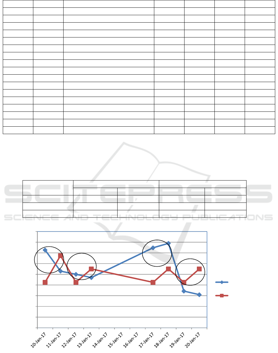
Figure 1. Comparison Actual and Predicted JSX Index before Modification

5220

5230

5240

5250

5260

5270

5280

5290

5300

5310

Actual

Predicted

BICESS 2018 - Borneo International Conference On Education And Social

426

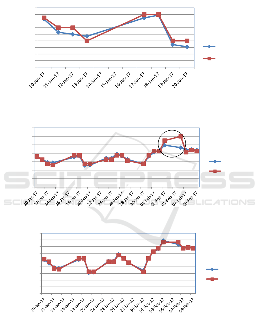
Figure 2. Comparison Actual and Predicted JSX Index after Modification

Figure 3. Comparison Actual and Predicted LQ-45 Index Before Modification

Figure 4. Comparison Actual and Predicted LQ-45 Index after Modification

Based on Figure 1 and Figure 3 shows that

the stock value of JSX and LQ-45 before the

modification still showed some significant variances

and can decrease the value of forecasting accuracy

index value. However, this is not shown in figure 2

and figure 4 that do forecasting with technical

5220

5230

5240

5250

5260

5270

5280

5290

5300

5310

Actual

Predicted

850

860

870

880

890

900

910

920

Actual

Predicted

860

865

870

875

880

885

890

895

900

905

Actual

Predicted

Econometric: Modiﬁcation Technique of Fuzzy Time Series First Order and Time-invariant Chen and Hsu to Increase the Forecasting

Accuracy of Value Stock Index in Indonesia

427

modifications and line index value between actual

and predicted tends to coincide and be able to follow

the pattern of the value of stock index JSX and LQ-

45.

4 CONCLUSIONS

This research showed that the index of JSX after

using the technique of a modified fuzzy time series

is able to provide value Mean Square Error (MSE) =

0.476, and Average Forecasting Error (AFER) =

0.0081% where the obtained value is much lower

than is possible using Fuzzy Time Series unmodified

(MSE = 3,782 and AFER = 0.0685%). On the index

of LQ-45, the modified fuzzy time series technic is

able to provide the MSE = -0.0449 and AFER =

0.0120% which is also lower than the prediction

using the technique of fuzzy time series unmodified

(MSE = -0.419 and AFER = 0.114% ). The results

of this research have found that the modification of

fuzzy time series at intervals redivided step able to

provide better forecasting accuracy.

REFERENCES

Chen, S. M. 2002. Forecasting Enrollments Based On

High-Order Fuzzy Time Series. Cybernetics And

Systems: An International Journal. 33: 1-16.

Chen, S.M dan Hsu, C.C. 2004. A New Method to

Forecast Enrollments Using Fuzzy Time Series.

International Journal of Applied Science and

Engineering 2 (3). pp : 234-244.

Chen. 1996. Chen, S. M. 1996. Forecasting Enrollments

Based On Fuzzy Time Series. Fuzzy Sets And Systems.

81. pp: 311-319.

Cheng, C.H., Chen, T.L., dan Teoh, H.J., 2008. Fuzzy

time series based on adaptive expectation model for

TAIEX forecasting. International Journal of Expert

System with Application. 34 (2008). pp : 1126-1132

Elfajar, A. B., Setiawan, B. D. dan Dewi, C. 2017.

Peramalan Jumlah Kunjungan Wisatawan Kota Batu

Menggunakan Metode Time Invariant Fuzzy Time

Series. Jurnal Pengembangan Teknologi Informasi

dan Ilmu Komputer. 1 (2). pp : 85-94.

Fauziah, N. Wahyuningsih, S., and Nasution, Y.N. 2016.

Peramalan Mengunakan Fuzzy Time Series Chen

(Studi Kasus: Curah Hujan Kota Samarinda). Jurnal

Statistika. 4(2). pp : 52 – 61.

Google Finance. www. Google.com/finance. Accesed on

August 10

, 2017.

Handayani, L., dan Anggriani, D. 2015. Perbandingan

Model Chen Dan Model Lee Pada Metode Fuzzy Time

Series Untuk Prediksi Harga Emas. Jurnal

Pseudocode. 2 (1). pp : 28 – 36.

Hansun, S. 2012. IHSG Data Forecasting Using Fuzzy

Time Series. Indonesian Journal Of Computer and

Cybernetics System. 6 (2) : 79 – 88.

Hasudungan, F. I., Umbara, R. F dan Triantoro, D. 2016.

Prediksi Harga Saham Dengan Metode Fuzzy Time

Series dan Metode Fuzzy Time Series-Genetic

Algorithm (Studi Kasus: PT Bank Mandiri (persero)

Tbk). e-Proceeding of Engineering : 3 (3). pp : 5372 -

5377.

Huarng, K.H. and Yu, K. 2006. The application of neural

networks to forecast fuzzy time series. Physica A:

Statistical Mechanics and its Applications. 363(2). pp

:481–491

Jilani, T. A., Burney, S. M. A., dan Ardil, C. 2007. Fuzzy

Metric Approach for Fuzzy Time Series Forecasting

Based on Frequency Density Based Partioning.

Proceedings of world journal academy of science,

engineering and technology, 23. pp : 333-338.

Rahmadiani, A., and Wiwik, A. 2012. Implementasi Fuzzy

Neural Network Pasien Poli Bedah di Rumah Sakit

Onkologi Surabaya. Jurnal Teknik ITS. 1 (1). pp : 403-

407.

Rukhansah, N., Muslim, M. A., and Arifudin, R. 2015.

Fuzzy Time Series Markov Chain Dalam Meramalkan

Harga Saham. Proceedings of the National Seminar on

Computer Science (SNIK 2015). pp : 309-321.

Song, Q. dan Chissom, B. S. 1993. Forecasting

Enrollments With Fuzzy Time Series － Part I. Fuzzy

Sets and Systems. 54. pp : 1-9.

Stevenson, M. dan Porter, J.E. 2009. Fuzzy Time Series

Forecasting Using Percentage Change as the Universe

of Discourse, World Academy of Science, Engineering

and Technology, 27(55). pp : 154-157.

Sullivan, J. and Woodall, W. H. 1994. A Comparison Of

Fuzzy Forecasting And Markov Modeling. Fuzzy Sets

and Systems. 64. pp: 279-293

Zulfikar, R. and Mayvita, P.A., 2017. Pengujian Metode

Fuzzy Time Series Chen dan Hsu Untuk Meramalkan

Nilai Indeks Bursa Saham Syariah Di Jakarta Islamic

Index (JII). WIGA-Jurnal Penelitian Ilmu

Ekonomi, 7(2). pp : 108-124.

BICESS 2018 - Borneo International Conference On Education And Social

428