
Stability Analysis of Cycle Business Investment Saving-Liquidity
Money (IS-LM) Model using Runge-Kutta Fifth Order and Extended
Runge-Kutta Method
Ulia Maulidah Musyaffafi
1
, Mohammad Hafiyusholeh
1
, Yuniar Farida
1
, Aris Fanani
1
and Ahmad Zaenal Arifin
2
1
Sunan Ampel Islamic State University, Street Ahmad Yani 117, Surabaya, East Java, Indonesia
2
Universitas PGRI Ronggolawe, Tuban, East Java, Indonesia
Department of Mathematics, Science and Technology
az_arifin@unirow.ac.id
Keywords: Routh-Hurwitz Criteria, Runge-Kutta Fifth Order, Extended Runge-Kutta.
Abstract: Forecasting the future conditions of economic stability can be illustrated in business cycle model. The IS-LM
business cycle model is a business cycle model which is represented in a differential equation involving
investment function (I), saving function (S), and money demand function (L). In this research, stability
analysis on the IS-LM business cycle model was performed. Stability analysis was performed by Routh-
Hourwitz criteria. After that, numerical simulation would be performed by comparing the Runge-Kutta
method of fifth order and Extended Runge-Kutta to determine the stability speed of the model. This research
resulted fixed point IS-LM model that is
∗
,
∗
,
∗
0.0979,0.0097,0.0351. Through data
simulations, it was obtained numerical solution with the Extended Runge-Kutta method that has faster stable
result, with25, compared with the Runge-Kutta Fifth Order method that is stable when 36.
1 INTRODUCTION
Indonesia is one of the countries that has experienced
economic crisis since the 1990s. Until now, the state
of the economy has been fluctuating and tends to be
unstable. One example of economic growth in
Indonesia in 2018 was overshadowed by a slowdown
compared to previous year. As for information, in
2017 Indonesia economic growth reached 5.07% or
lower than the growth of neighboring countries, such
as Malaysia which has 5.8% growth (Angriani, 2018).
This situation requires Indonesia to develop
economic forecasting in order to know the future
condition of the economy.
Forecasting future economic conditions can be
illustrated in the business cycle models, one of which
is the IS-LM (Investment Saving-Liquidity Money)
business cycle model. The IS-LM business cycle
model is a system of differential equations involving
the investment function (I), the saving function (S),
and the money demand function (L) (Dwiningtias &
Abadi, 2014).
The IS-LM business cycle model is a business
cycle model that is represented in the form of a system
of differential equations (Dwiningtias & Abadi,
2014). The method used in solving differential
equation can be obtained by analytical or numerical
method. However, the weakness of the analytical
method is that not all mathematical equations can be
solved to produce the exact value and the method
takes a very long time in the process of work
(Alfaruqi, 2010). Therefore, numerical methods are
needed as alternative to analytical methods. The
numerical methods in question include Taylor series
method, Euler method, Runge-Kutta method, and
Heun method. Meanwhile, methods that include
many steps are Adam-Bashforth-Moulton method,
Milne-Simpson method, and Hamming method.
Among these methods, researchers are more
interested in using the fifth order Runge-Kutta
method and the Extended Runge-Kutta Method to
look at the behavior of dependent variables that affect
the business cycle model. The advantage of the
Runge-Kutta method is that it does not use derivatives
in its process (Muhammad, 2015). In addition, the
240
Musyaffafi, U., Hafiyusholeh, M., Farida, Y., Fanani, A. and Arifin, A.
Stability Analysis of Cycle Business Investment Saving-Liquidity Money (IS-LM) Model using Runge-Kutta Fifth Order and Extended Runge-Kutta Method.
DOI: 10.5220/0008905400002481
In Proceedings of the Built Environment, Science and Technology International Conference (BEST ICON 2018), pages 240-246
ISBN: 978-989-758-414-5
Copyright
c
2022 by SCITEPRESS – Science and Technology Publications, Lda. All rights reserved

higher the order is used, the greater the level of
accuracy produced.
This research is interesting because the IS-LM
cycle model will be stability analysis of the model and
model simulation is performed to show the behavior
of variables affecting IS-LM business cycle model in
graphic form. In addition, a comparison of the fifth
order Runge-Kutta method and the Extended Runge-
Kutta Method will be used to simulate the model that
has been obtained with the stability speed of the
model.
This research will be stability analysis of IS-LM
business cycle model with variable of income rate,
rate of interest, and capital stock rate. This model is a
modified model of the business cycle model of
Gabisch and Lorenz (1987) by substituting
investment, saving, and money demand functions.
Model stability analysis was performed by
determining fixed point which then performed fixed
point stability analysis with Routh-Hurwitz criteria
followed by determining stability time through
Runge-Kutta method of order five and Extended
Runge-Kutta.
2 THEORITICAL FRAMEWORK
2.1 Business Cycle Model
The IS-LM model is one of the models in the field of
macroeconomics. The IS-LM business cycle model
involves investment (saving) function, saving
function on goods market and Liquidity preference,
and Money supply in money market (Rosmely, et al.,
2016).
The business cycle model was first introduced by
Kalecki (1935) and Kaldor (1940) in the form of a
system of differential equations, ie.:
,
,
,
(1)
with
is the rate of income,
is the rate of capital
stock,
,
is an investment function that
relies on income and capital stock,
,
is a
saving function that depends on income and capital
stock, and 0 is the acceleration due to the excess
or lack of investment.
In 1977, Torre changed the model (1) by
replacing the capital stock (K) variable with the
interest rate variable (R). The business cycle is
modelled as follows:
,
,
,
(2)
with
is the interest rate,
,
is a money
demand function that depends on income and interest
rates, 0 is the acceleration caused by the lack or
excess demand for money, and 0 is the constant
supply of money.
Then in 1987, Gabisch and Lorenz added capital
stock variables (K) into the business cycle model (2),
so that it becomes a business cycle model
,
,
,
,
(3)
,
,
with 0 is the capital depreciation constant.
2.2 Function I,S, and L
In 2005, Cai provided assumptions on the investment
function (I),saving function (S) and money demand
functions (L). The amount of investment (I) islinearly
dependent on the difference between income (Y)
subtracted by capital stock (K) and interest rate (R).
Meanwhile, the saving function (S) depends on the
sum of income (Y) with interest rate (R). Money
demand functions (L) depends on the difference
between income (Y) and interest rate (R). All three
functions can be denoted as follows:
,,
,
(4)
,
Annotation,
growth rate of investment to income,
the rate of decline in investment on capital stock,
growth rate of savings to income,
the growth rate of money demand for income,
the rate of decline in investment on interest
rates,
the growth rate of savings on interest rates,
the rate of decline in demand for money against
interest rates,
where ,
,
,
,
,
,
are positive constants in
the interval
0,1
.
2.3 Matrix Jacobi
In searching for stability analysis, it is necessary to
have a characteristic equation on differential
equations constructed from a Jacobi matrix.
Stability Analysis of Cycle Business Investment Saving-Liquidity Money (IS-LM) Model using Runge-Kutta Fifth Order and Extended
Runge-Kutta Method
241

Given functionality
,
,
,…,
in
system with
∈,1,2,…,.
⋯
⋮⋱⋮
⋯
6
Matrix above is called the Jacobian matrix of at
point (Hale & Kocak, 1991).
2.4 Eigen Value
If is a matrix x , then a nonzero vector in
called the eigenvector of
if is a scalar multiple
of
, i.e.
(7)
For any scalar
, scalar is called the eigenvalue
of
, and is called the eigenvector of which is
related
(Rosmely, Nugrahani, & Sianturi, 2016).
To obtain the eigenvalues of a matrix
,
equation (7) can be rewritten as
or equivalent to
0 (8)
So can be an eigenvalue. There must be a non
zero solution of the equation (8). Equation (8) has a
non zero solution if and only if
0 (9)
Equation (9) is called characteristic equation of
matrix . Scalars keeping the equation (9) are
eigenvalues
(Anton, 2008).
2.5 Routh-Hurwitz Criteria
One of the methods that can be used in determining
fixed point stability is the Routh-Hurwitz stability
criterion, which is a criterion for showing stability by
not seeing the real sign of the eigen value directly but
by looking at the coefficients of the characteristic
equation. The Routh-Hurwitz Stability Criteria is
expressed in Theorem 1 below:
Theorem 1. Example
,
,…,
real numbers
0 if . All values of the characteristic
equation
⋯
0
And Hurwitz matrix as follows:
1
…0
…0
0
01
…0
…0
⋮⋮⋮
⋮⋱⋮
…
Then the eigenvalue of the equation
(9) will have
a negative real part if and only if the determinant of
the matrix
is positive:
0 for all 1,2,…,
According to Routh-Hurwitz criteria, the above
theorem for value 2,3,4, , the fixed point will be
stable if and only if:
2;
0,
0
3;
0,
0,
,
4;
0,
0,
0,
2.6 Runge-Kutta Method of the Fifth
Order
The Runge-Kutta method is a development of the
Euler method with the completion calculation
performed step by step (Alfaruqi, 2010). This method
is an alternative to the Taylor series method that does
not require derivative calculations (Iffatul, 2016).
However, not all functions can be easily counted. The
higher the order in the Taylor series is, the higher the
derivative should be calculated and it makes the
Taylor series rarely used in the solution of ordinary
high-order differential problems (Alfaruqi, 2010).
The fifth order Runge-Kutta method can be written as
follows:
4
(10)
with:
,
1
3
,
1
3
1
3
,
1
6
1
6
1
2
,
1
8
3
8
,
1
2
3
2
2
2.7 Extended Runge-Kutta Method
The Extended Runge-Kutta method is an extension of
the Runge-Kutta method on the main function and its
evaluation function (Muhammad, 2015). In general,
the Extended Runge-Kutta equation model can be
written as follows:
∑
(11)
with,
,
′
,
BEST ICON 2018 - Built Environment, Science and Technology International Conference 2018
242

Equation (11) is a major function of the general
equation of Extended Runge-Kutta model. So that
equation of Extended Runge-Kutta fourth order is can
be obtained as follows:
(12)
with,
,
,
,
,
′
,
′
,
′
,
′
,
3 METHODOLOGY
3.1 Type of Research
This research is a quantitative research because this
research used quantitative data so that data analysis
used quantitative analysis.
3.2 Variable of Research
In this research, variables consist of independent
variables and dependent variables. The independent
variables used are the acceleration due to
excess/shortage of investment stock, the constant of
money supply, the acceleration due to
excess/shortage of money demand, the constant of
capital depreciation, the rate of investment growth on
capital stock, the level of investment to income, the
growth rate of savings to income, money to earnings,
decreased demand for money on interest rates,
reduced rates of investment on interest rates, and
growth rates on savings on interest rates.
Meanwhile, the dependent variables used are the
national income rate, the rate of interest rate, and the
rate of capital stock. The variables used in this
research are secondary data obtained from Bank
Indonesia in 2016.
3.3 Method of Research Analyze
The process of analysis in this research is divided into
two, namely:
a. Analysis of fixed point stability of IS-LM model
The algorithm for performing fixed point
stability analysis of IS-LM model as follows:
1. Determining the IS-LM model used by
substituting the Gabisch-Lorenz IS-LM
model into the investment, saving, and
money demand functions of Cai. (Equation
(4)).
2. Determining the fixed point of the IS-LM
model using the method of elimination and
substitution to obtain the point
∗
,
∗
, and
∗
.
3. Determining Jacobi's matrix in Equation (6).
4. Determining characteristic equation that
fullfills det
0.
5. Determining the stability of fixed points
through Routh-Hurwitz criteria
b. Numerical simulation of the IS-LM model
1. Variable declarations used in the IS-LM
business cycle model
(,
,
,
,
,
,
).
2. Determining a numerical solution using
the fifth-order Runge-Kutta method
3. Determining the stability time of each
method
4. Determining the best method of both
methods according to the fixed point
stability time velocity.
4 ANALYSIS AND DISUSSION
4.1 Model Stability Analysis
The business cycle model used in this research was a
model introduced by Gabisch and Lorenz (1987) by
substituting the investment, saving, and capital stock
functions of equation (4) into equation (3) with the
parameters given by Cai ( 2005), namely:
(13)
with ,
,
,
,
,
,
are positive constants in
the interval
0,1
.
The fixed point in the equation (13) can be
obtained if it fulfills
0.
so it obtains
0 (14)
0 (15)
0 (16)
Next is to find fixed point
∗
,
∗
,
∗
by using
elimination and substitution on each equation.
Stability Analysis of Cycle Business Investment Saving-Liquidity Money (IS-LM) Model using Runge-Kutta Fifth Order and Extended
Runge-Kutta Method
243

Thus, fixed point model, that is
∗
,
∗
,
∗
,
was obtained where:
∗
∗
(17)
∗
The stability of the fixed point is obtained by
looking at the eigenvalues of the characteristic
equations derived from the model by searching
(0, so we can get the characteristic
equation
0 (18)
when
Because the eigenvalues of the equations (18) was
difficult to determine, the stability of the fixed point
can be investigated using the Routh-Hurwitz
criterion. According to Routh-Hurwitz criteria, the
eigenvalues of the equation (18) will make a fixed
point
∗
,
∗
,
∗
(4.12) stable if and only if
0,0,and 0.
4.2 Numerical Simulation using
Runge-Kutta Method of the Fifth
Order
In this section, a numerical simulation of the IS-LM
business cycle model will be conducted to find the
stability time of the model using the Runge-Kutta
method of order five.
The initial value used in the simulation was data
from Bank Indonesia in 2016 in the form of income
rate 5, rate of interest 9.18, and
capital stock rate 4.47 [9]. The parameters
used in the simulation of this business cycle model
are presented in Table 1.
Based on these parameters and by taking into
account the data in Table 1, it was obtained a fixed
point
∗
,
∗
,
∗
0.0979,0.0097,0.0351.
Before performing numerical simulations, a fixed
point stability simulation was performed by
substituting the parameters in Table 1 into equations
(18). It will be shown that the parameter meets Routh-
Hurwitz criteria such that the point remains stable.
Table 1: Value of business cycle parameters.
Symbol Parameter Definition Value
The growth rate of investment to
income
0.5
The rate of decline in investment on
capital stock
0.7
Constant depreciation of capital
0.5
Saving growth rate against income
0.1
The growth rate of money demand fo
r
income
0.6
The rate of decline in investment on
interest rates
0.7
The rate of saving growth against
interest rates
0.8
The rate of decline in money demand
on interest rates
0.9
Constant money supply
0.05
Acceleration due to the excess or lac
k
of investment
1
Acceleration due to the excess or lac
k
of money demand
4
According to Routh-Hurwitz criteria, the point
remains stable if and only if 0,0, and
0. The simulation results based on these criteria
can be seen in Table 2.
Table 2: Eigen Value of Characteristic Equations.
4.4000
6.3500
2.6760
25.2640
Based on the table above, it can be seen that the
eigenvalue of the characteristic equation in equation (18)
satisfied the Routh-Hurwitz criterion 4.4000
0,2.67600, and 25.26400 so
the fixed point of the model was stable.
The next was to develop numerical simulation
with the Runge-Kutta method of order five with the
help of MATLAB R2013 software by substituting the
parameters in Table 1 into Eq. (13) to obtain the graph
in Figure.1.
Figure 1: Numerical simulation by Runge-Kutta method of
the fifth order.
BEST ICON 2018 - Built Environment, Science and Technology International Conference 2018
244
The business cycle will experience different
fluctuations and then move constantly to a fixed point
so as to obtain a stable point. Figure 1 shows business
cycle stability around the point. Figure 1 shows
business cycle stability around the point 36 with
value 0.0979,0.0097, and 0.0351.
Therefore, according to Routh-Hurwitz criteria, this
business cycle is stable.
4.3 Numerical Simulation with
Extended Runge-Kutta Method
The initial value used in this simulation was the same
as the previous simulation of the income rate
5, rate of interest 9.18, and capital stock rate
4.47. The resulting numerical simulation is
as follows.
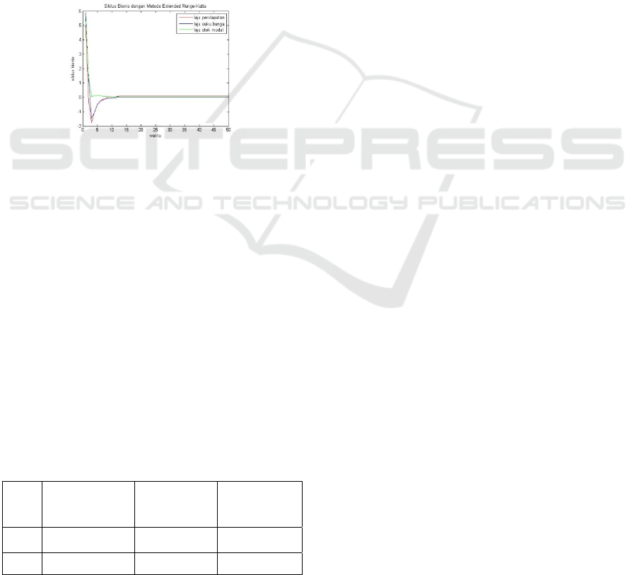
Figure 2: Numerical simulation with Extended Runge-
Kutta method.
Based on Figure 2,. the business cycle model with
the Extended Runge-Kutta method has similar pattern
and behavior that decrease (recess) and then move
constantly to a stable point. In Figure 2, the business
cycle has stability around the point 25 with value
0.0979,0.0097, and 0.0351.
Therefore, according to Routh-Hurwitz criteria, this
business cycle is stable.
4.4 Comparison Method
In this research, the comparison of the two methods
was developed by comparing the stability time of
each method and computation time to obtain a stable
point.
Table 3: Comparison Method.
Income Rate
(0.0979)
Rate of
Interest (
0.0097)
Capital Stock
Rate (
0.0351)
RK5
36 35 32
ERK
25 25 24
Based on Table 3, we can shows the stability time
of each method. The stability time resulting from the
Runge-Kutta method of order five was the rate of
income that was stable at 36, rate of interest that
had stable moment 35, and the capital stock rate
that was stable at the moment 32. Meanwhile, the
stability time generated by the Extended Runge-Kutta
method was the income rate that was stable at the
moment 25, rate of interest that was stable at the
moment 25, and the capital stock rate that was
stable at the moment 24.
Based on the Runge-Kutta method, the fifth order
business cycle model will experience stability in the
next 36 years, or in 2052, and with the Extended
Runge-Kutta method, stability of the next 25 years
will be in the year 2041. Both will be stable at the
point
∗
,
∗
,
∗
0.0979,0.0097,0.0351
.
Therefore, the Extended Runge-Kutta method has
a faster stability time than the Runge-Kutta method.
This is because the main function of the Extended
Runge-Kutta is added with the derivative function.
So, the results obtained by the Extended Runge-Kutta
method are faster to be stable than the fifth order
Runge-Kutta method.
5 CONCLUSIONS
Based on the formulation of the problem and the
results of the discussion, the following conclusions
can be obtained:
1. In the IS-LM business cycle model, we get a
stability model of equilibrium point
∗
,
∗
,
∗
0.0979,0.0097,0.0351. Model
of business cycle stability can be shown by the
value of the equation of characteristics obtained
from the model, that is
0
with
By substituting the parameter values, it was
obtained 4.40000,2.67600, and
25.26400 which meets the Routh-
Stability Analysis of Cycle Business Investment Saving-Liquidity Money (IS-LM) Model using Runge-Kutta Fifth Order and Extended
Runge-Kutta Method
245

Hurwitz criteria so that the IS-LM business cycle
model is stable.
2. The numerical solution using the Runge-Kutta
method of order five obtained the time stability of
the IS-LM business cycle model by substituting
the parameters when 36.
3. Numerical solution using Extended Runge-Kutta
method obtained the time stability of the IS-LM
business cycle model by substituting the
parameters when 25.
4. In determining the stability of the IS-LM model,
the Extended Runge-Kutta method has a faster
stability time with 36 than the current fifth
order Runge-Kutta method with 25. This
happens because the Extended Runge-Kutta
method adds the derivation function to the main
function so that the stability point gets faster.
REFERENCES
Alfaruqi, 2010. Penyelesaian Persamaan Diferensial Biasa.
Pens Its, Pp. 65-75.
Angriani, D., 2018. metroTVnews.com. [Online] Available
at: http://ekonomi.metrotvnews.com [Accessed 1 2
2018].
Anonim, n.d. https://kbbi.kata.web.id/pertumbuhan-
ekonomi/. [Online] [Accessed 28 03 2018].
Anton, H., 2008. Aljabar Linier Elementer. Jakarta:
Erlangga.
Cai, J., 2005. Hopf bifurcation in the IS-LM business cycle
model with time delay.. Electronic Journal of
Differential Equations., pp. 1-6.
Chapra & Canale, 1990. Numerical methods for engineers.
New York: McGraw-Hill Book Co..
Dernburg, T. F. & Muchtar, K., 1987. Makroekonomi edisi
ketujuh. Jakarta: Erlangga.
Dornbusch, Rudiger & Fisher, 2016. Ekonomi makro.
s.l.:s.n.
Dwiningtias & Abadi, 2014. Model siklus bisnis dengan
waktu tundaan. MATHunesa.
Gabisch, G. & Lorenz, H.-W., 1989. Business Cycle
Theory A Survey of Methods and Concepts. Springer.
Hale, J. K. & Kocak, H., 1991. Dynamic and Bifurcation.
Springer-verlag.
Iffatul, 2016. gunadarma.ac.id. [Online] Available at:
iffatul.staff.gunadarma.ac.id/.../BAb-
+08+Solusi+Persamaan+Diferensial+Biasa.pdf
[Accessed 21 Januari 2018].
Indonesia, B., 2017. Laporan Perekonomian Indonesia.
Jogiyanto, H., 2006. Metodologi Penelitian Bisnis. BPFE
UGM.
Kaddar, A. & Alaoui, H. T., 2008. Fluctuation in a Mixed
IS-LM Business Cycle Model. Electronic Journal of
Differential Equations, pp. 1-9.
Kaldor, N., 1940. A Model of the Trade Cycle. JSTOR, pp.
78-92.
Kalecki, M., 1935. A Macrodynamic Theory of Business
Cycles. JSTOR, pp. 327-344.
Lestari, E. P., 2011. Intensitas Perdagangan dan
Keselarasan Siklus Bisnis di ASEAN-4 dan UNI-
EROPA. Jurnal Ekonomi Pembangunan, pp. 163-186.
Luenberger, D., 1979. Introduction to Dynamic Systems.
New York: Wiley.
Mankiw, G., Quah, E. & Wilson, P., 2012. Pengantar
ekonomi makro. Jakarta: Salemba Empat.
Mardiana, A., 2014. Uang dalam ekonomi islam. Al-
Buhuts, Volume 10, p. 91.
Muhammad, S. T., 2015. Pengkajian metode extended
runge kutta dan penerapannya pada persamaan
diferensial biasa. JURNAL SAINS DAN SENI ITS, pp.
Vol. 4, No.2, (2015) 2337-3520.
MZI, 2015. Telkom University. [Online] Available at:
http://cdndata.telkomuniversity.ac.id [Accessed 2 Mei
2018].
Pasaribu, R. B. F., 2009. Fluktuasi Ekonomi Dan Siklus
Ekonomi. Universitas Gunadarma, pp. 1-61.
Reksoprayitno, S., 2012. Pengantar Ekonomi Makro.
Yogyakarta: BPFE-Yogyakarta.
RI, K., 2015. Qur'an Kemenag, Jakarta: Kementrian
Agama.
Rosmely, Nugrahani, E. H. & Sianturi, P., 2016. Analisis
Bifurkasi Pada Model Siklus Bisnis Is-Lm (Investment
Saving-Liquidity Money). IPB Repository.
Samuelson, P. A. & Nordhaus, W. D., 1997.
Makroekonomi. Jakarta: Erlangga.
Sugianti, D., 2017. Analisis Model Matematika Order
Fraksional Makroekonomi Investment Saving-Liuidity
Money (IS-LM) di Indonesia. Airlangga.
Suparmoko, 2000. Keuangan Negara. BPFE.
Supriyono & Miyoshi, T., 2014. Perbandingan algoritma
metode MECD dan metode runge-kutta untuk
menyelesaikan persamaan diferensial berderajat dua
yang bersistem besar. pp. 149-158.
Torre, V., 1977. Existence of limit cycles and control in
complete Keynesian. JSTOR, pp. 1457-1466.
Umar, M., 2009. Analisis Dampak Kebijakan Fiskal dan
Moneter dalam Perekonomian Indonesia: Aplikasi
Model Mundell-Fleming. Diponegoro.
BEST ICON 2018 - Built Environment, Science and Technology International Conference 2018
246
