
Possible Method for Monthly Natural Rubber Price Forecasting
Ketut Sukiyono
1*
, Nusril
1
, Eko Sumartono
1
, Indra Cahyadinata
1
, M. Zulkarnain Yuliarso
1
, Gita
Mulyasari
1
, Musriyadi Nabiu
1
, Febrina Nur Annisa
2
1
Department of Agricultural Socio-Economics, Faculty of Agriculture, University of Bengkulu
2
Study Program of Magister of Agribusiness Management Faculty of Agriculture, University of Bengkulu
Keywords : Rubber, Double Exponential Smoothing, Decomposition, ARIMA, forecasting.
Abstract : Future price information is crucial not only for producers but also for other agribusiness actors. Price is a
signal for them to make a decision regarding what to produce and when to sell including for natural rubber.
For this reason, forecasting and selecting the best model becomes important. This study is aimed to
analyze and select the possible forecasting methods for monthly natural rubber prices in Indonesia and
World Markets. The univariate model of Double Exponential Smoothing, Decomposition, and ARIMA
models are applied to forecast price data from 2012:1 – 2016:12. The selection of an accurate model is
based on the lowest value of MAPE, MSD, and MAD. ARIMA is the possible methods for world rubber
price forecasting while Double Exponential Smoothing should be applied for predicting domestic rubber
prices because it allows for better predictive performance.
1 INTRODUCTION
Price is often used as a signal for producers to
produce and or sell a commodity. Ribeiro, Sosnoski,
and Oliveira (2010) stated that decision making
requires information on how prices behave before
the harvest is done. In addition, price fluctuations
make agriculture a risky business as reported by
Grega (2002) and Fafchamps (2000). Price is also
often a determinant of the level of competitiveness
of a product. Therefore, price determination will be
able to assure the sustainability of farm business
including rubber farming. Price uncertainty also
causes difficulties in designing policies related to
improving the welfare of farmers. Price uncertainty
and price volatility also make farmers more
vulnerable (FAO et al., 2011 and Sukiyono, et al.,
2017) in the case of oil palm farmers). With these
environmental conditions, price information in the
future will be very important. Future pricing
information requires accurate price forecasting. Any
error in the prediction of price can cause a huge
amount of revenue loss. This implies the importance
of selecting the most probable forecasting model.
Several analytical methods for forecasting are able
to apply. Pandey and Upadhyay (2016) classify
these forecasting methods into two categories: time
series and simulation approach. Kirchgassner and
Wolters (2007) and Pandey and Upadhyay (2016)
state that a time series is defined as a set of
numerical observations arranged in sequenced order
or an even time interval. These data are historical
data from market prices and collected at an equally
spaced and discrete time interval. On the other hand,
the simulation approach requires and generates a
large amount of data and computationally intensive.
This current paper applies a time series approach
and is aimed at selecting a possible method for
forecasting rubber price at world and domestic
(Indonesia) markets.
Among time series forecasting models, three
models are commonly used, that is, exponential
smoothing, decomposition, and ARIMA.
Exponential Smoothing method is designed based on
a simple statistical model and does not use any
variable other than the variable being forecast.
Robert and Amir (2009) note that the exponential
smoothing model has advanced significantly in the
last few decades and established as one of the
forecasting methods. Sudha et al., (2013) and Rani
and Raza (2012) are among researchers using
exponential smoothing models to forecast
agricultural product and price. Another time series
forecasting model is a decomposition approach.
This approach involving additive and multiplicative
decomposition separates trend and seasonal
172
Sukiyono, K., Nusril, ., Sumartono, E., Cahyadinata, I., Yuliarso, M., Mulyasari, G., Nabiu, M. and Annisa, F.
Possible Method for Monthly Natural Rubber Price Forecasting.
DOI: 10.5220/0008785301720179
In Proceedings of the 2nd International Research Conference on Economics and Business (IRCEB 2018), pages 172-179
ISBN: 978-989-758-428-2
Copyright
c
2020 by SCITEPRESS – Science and Technology Publications, Lda. All rights reserved

component from time series and computes the
prediction whether by multiplying or adding to
seasonal indices Saini, Saxena, and Surana (2017).
This model has applied for various agricultural
products, among others are Taru and Mshelia (2009)
and Bergmann, O’Connor and Thümmel (2015). A
comprehensive discussion on decomposition method
is given by Dogum (2010) and Prema and Rao
(2015). Finally, an Auto-Regressive Integrated
Moving Average (ARIMA) model, introduced by
Box and Jenkins (1976), is a technique for finding
the most suitable pattern from a group of time series
data, by utilizing past and present data to perform
accurate forecasting. Weiss (2000) defines that
ARIMA is a linear function of the previous actual
values and random shocks. This model is also
widely used in various agricultural products prices,
such as chicken, pork, cabbage and other major
agricultural prices (Hu Tao (2005) and Feng Liu et
al. (2009)).
Each forecasting method discussed above also
shows the advantages and disadvantages of each
method. The problem is what the most accurate
forecasting model for forecasting rubber prices in
both the world market and the domestic market is.
The selection of forecasting models so far has
tended to use subjectivity considerations. There is no
explanation from researchers regarding the selection
and application of certain forecasting models for
their research. Some researchers have tried to choose
the best forecasting model using several models,
including Sukiyono and Rosdiana (2018) on the
price of rice at the wholesale level. From some of
these studies, each different commodity and
observation period has the best different model. That
is, the forecasting model for commodities will not
necessarily be appropriate or accurate for other
commodities. Therefore, this study tries to determine
the best model by comparing the accuracy of
forecasting from the three models that are widely
used so far, namely double exponential smoothing,
decomposition, and ARIMA.
2 METHODS
This research used monthly data on rubber prices at
domestic and world markets from 2012:1 – 2016:12
or 72 observations. Three-time series forecasting
models are proposed namely, double exponential
smoothing, additive and multiplicative
decomposition, and ARIMA. These methods are
explained in brief as follows:
2.1 Double Exponential Smoothing
Exponential Smoothing Model is a continuous
improvement procedure for forecasting against the
latest observational objects to produce a smoothed
time series (Kumar and Gwada, (2015) and Jatra
(2013)). This model focuses on exponentially
decreasing weights as the observation get older. In
other words, recent observations are given relatively
more weight in forecasting than the previous
observations.
This study applies double exponential
smoothing, also known as trend adjusted exponential
smoothing. This model departs from improving a
single exponential smoothing model by introducing
the second equation with a second smoothing
constant or second weight (α
2
) and assuming
monthly rubber price is influenced by the trend
component. Kumar and Gwada, (2015) stated that
introduction and selection of (α
2
) having to consider
(α
1
). The double exponential model can be written
as follows:
1111
1
tttt
bSXS
(1) and
1212
1
tttt
bSSb
(2)
where,
t
S
= smoothened value at time period t;
1
t
S
= smoothened value at time period t – 1; α
1
=
level smoothing constant;
1
X
= actual price at time
period t;
t
b
= trend estimate of the time period
t;
1
t
b
= trend estimate of the period t-1; and α
2
=
trend smoothing constant.
2.2 Decomposition Method
Decomposition methods are based on an analysis of
the individual components of a time series, i.e.,
trend, seasonality, cycle, and error. In this
approach, each component strength is estimated
separately and then substituted into a model that
explains the behavior of the time series. There are
two decomposition methods: multiplicative and
additive (Peng and Chu, (2009) and (Rajchakit,
2017). An additive decomposition model takes the
following form:
ttttt
eS
C
TY
(3)
while a multiplicative decomposition model can be
written as:
ttttt
eS
C
TY
, (4)
where
t
Y
, the actual time series value at period t, is
a function of four components: seasonal (S),
Possible Method for Monthly Natural Rubber Price Forecasting
173
cyclical (C), the trend (T) and an error component
(e).
2.3 Arima
In applying an ARIMA model, this research follows
Box-Jenkins methodology which involves four
steps, namely identification, estimation, model
checking, and forecasting. Dieng (2008) explains
that the Box-Jenkins forecasting approach involves
an interactive process between the forecaster and the
data in terms of using diagnostic statistics to select
the appropriate models. This approach also requires
fewer data and has generally proved successful in
practice. In general, according to Ekananda (2014),
an ARIMA model is characterized by the notation
ARIMA (p, d, q), where p, d, and q denote orders of
Auto-Regression (AR), Integration (differencing)
and Moving Average (MA), respectively. ARIMA is
a parsimonious approach which can represent both
stationary and non-stationary processes. Box and
Jenkins (1976), an economic variable, Y, has a
generating function which belongs to ARIMA (p, d,
q) model is given by:
qtq1t1tptp1t11t1t
Y
Y
Y
Y
(5)
where t = 1, 2, 3 ... T
t
is an uncorrelated process
with mean zero,
i
and
i
are coefficients (to be
determined by fitting the model)
2.4 Forecasting Accuracy Measures
Three accuracy measures were calculated: Mean
Absolute Percentage Error (MAPE), Mean Absolute
Deviation (MAD), and Mean Squared Deviation
(MSD). MAPE is a percentage point error while
MAD and MSD are scale-dependent measures.
Karim, Awala and Akhter (2010) noted that the
smaller measurement values show more accurate
forecasts since it produces minimum forecasting
error. It should be noted that there was no shock
variable at the period of study. It means that there is
no unexpected change in a variable under analysis.
3 RESULTS AND DISCUSSION
3.1 Indonesian Rubber Profile
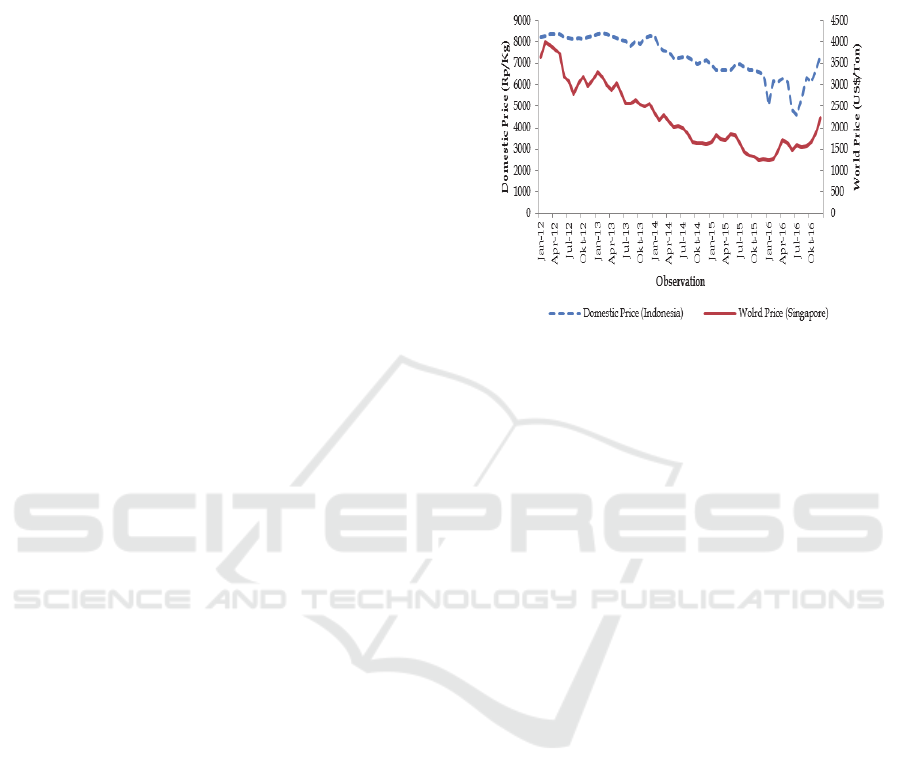
Figure 1: Domestic Rubber Price (Indonesia) and
World (Singapore).
Indonesian Rubber Production in 2015 amounted to
34,340 tons and is estimated continues to increase
until 2020 with a production of 40,449 tons (Karet
outlook 2016). In terms of consumption, rubber
consumption in 2020 is projected at 596 tons or
increase over the next five years with an average of
0.85% per year within the period 2016 - 2020. Karet
outlook (2016) also reported that for the next five
years Indonesia is expected to surplus Rubber. If in
2016 Indonesia's rubber surplus amounted to 35,575
tons, this surplus is projected to continue to increase
reaching 39,854 tons in 2020. The high production
of rubber in Indonesia places Indonesia as one of the
producers and exporters of rubber in the world.
Indonesia in 2010 only able to contribute to the
world rubber needs of 2.41 million tons of natural
rubber or second after Thailand which amounted to
3.25 million tons (Purba, 2011). In addition, based
on data from Perkebunan Perkebunan Nusantara, as
reported by (Kompas, 11/09/2017), rubber
production in Indonesia is currently recorded at 3.2
million tons per year. Of that amount, which can be
absorbed domestically only 18 percent and the rest
for export purposes. Indonesia's rubber exports are
mostly directed to Vietnam, the Netherlands, the
United States, and India.
Relation to the development of rubber prices,
domestic and world price data presented in Figure 1
show a reasonably fluctuating movement. Recorded
by Kompas, in 2011, the average price of rubber
reached 5.58 US dollars per kilogram (kg), whereas
IRCEB 2018 - 2nd INTERNATIONAL RESEARCH CONFERENCE ON ECONOMICS AND BUSINESS 2018
174
in 2017 the average is only 1.2 US dollars per kg in
the world market.
Figure 1 is not intended to compare the price
level at two markets due to different unit price, but it
is rather than to show the behavior pattern or
tendency of rubber price. Figure 1 shows that world
rubber prices and domestic rubber prices have likely
similar patterns. The price of rubber in both markets
tends to fall from the beginning of 2012 to the end of
2015 and started to increase in 2016. However, the
downward rubber price trend in the Singapore
market is sharper than in the domestic market.
Statistical summary of rubber price in domestic
and world markets is presented in Table 1. Table 1
shows that rubber prices in the domestic market in
the period January 2012 - 2016 moved from Rp
4,594.00/kg to Rp 8,408.00/kg with an average price
of Rp 7,288.42/kg and Standard Deviation of
967.81. While in the world market, prices move
from the US $ 1,230.00/ton to the US $ 4,000.00/ton
with an average price of US $ 2,260.00/ton.
Table 1: Statistical summary of Domestic and World
Rubber Price.
Level Mean St.
Dev.
Max Min
Domestic
Price
(Rp./Kg)
7,288,42
967.81
8,408.00
4,594.00
World
Price
(US$/To
n)
2,260.00
773.40
4,000.00
1,230.00
3.2 Model Forecasting Estimation
As discussed above, this article uses three
forecasting models, namely exponential smoothing,
ARIMA, and decomposition. The choice of the best
model is used by three indicators of the accuracy of
MAPE, MAD, and MSD where the model that has
the lowest MAPE, MAD, and MSD values shows
the most accurate forecasting method
3.3 Double Exponential Smoothing
This double exponential smoothing method uses two
smoothing coefficients namely α
1
(smoothing
constant) and α
2
(smoothing trend). This smoothing
coefficient is determined by trial and error to
produce the smallest error value (Stevenson, 2009).
An indicator used to select the values of α and β is
the Root Mean Square Error (RMSE), the best
values of α and β are indicated by the smallest
RMSE values. The results of forecasting rubber
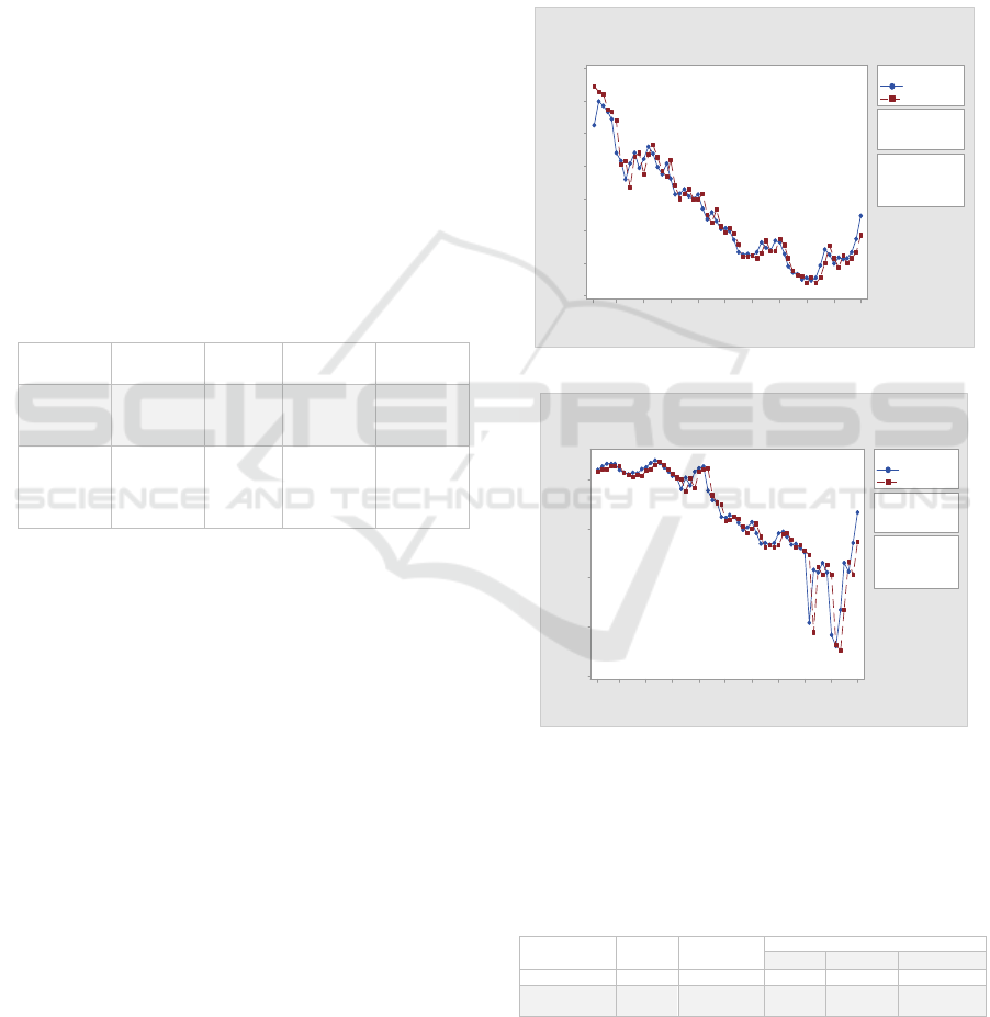
prices are presented in Figures 2 and 3, and Table 2.
For world rubber prices, the best values for α
1
and α
2
are 1.31913 and 0.02533 while for domestic
rubber prices, the best values are 1.07791 and
0.02571. Looking at these values, both show almost
the same value. This shows the similarity of data
patterns between the two markets (see Figure 2).
Table 2: Forecasting results using Double Exponential
Smoothing.
Prices
1
2
Accuracy Measure
MAPE MAD MSD
World Market 1.31913 0.02533 5.9 1.33 29,954.6
Domestic
Market
1.07791 0.02571 3.0 210.00 142,285.0
60544842363024181261
4500
4000
3500
3000
2500
2000
1500
1000
α (level) 1.31913
γ (trend) 0.02533
Smoothing Constants
MAPE 5.9
MAD 133.3
MSD 29954.6
Accuracy Measures
Index
World Price
Actual
Fits
Var iabl e
Smoothing Plot for World Price
Double Exponential Method
60544842363024181261
8000
7000
6000
5000
4000
α (level) 1.07791
γ (trend) 0.02571
Smoothing Constants
MAPE 3
MAD 210
MSD 142285
Accuracy Measures
Index
Domestic Price
Actual
Fits
Variable
Smoothing Plot for Domestic Price
Double Exponential Method
Figure 2: Smoothing Plots for World and Domestic
Price.
Possible Method for Monthly Natural Rubber Price Forecasting
175
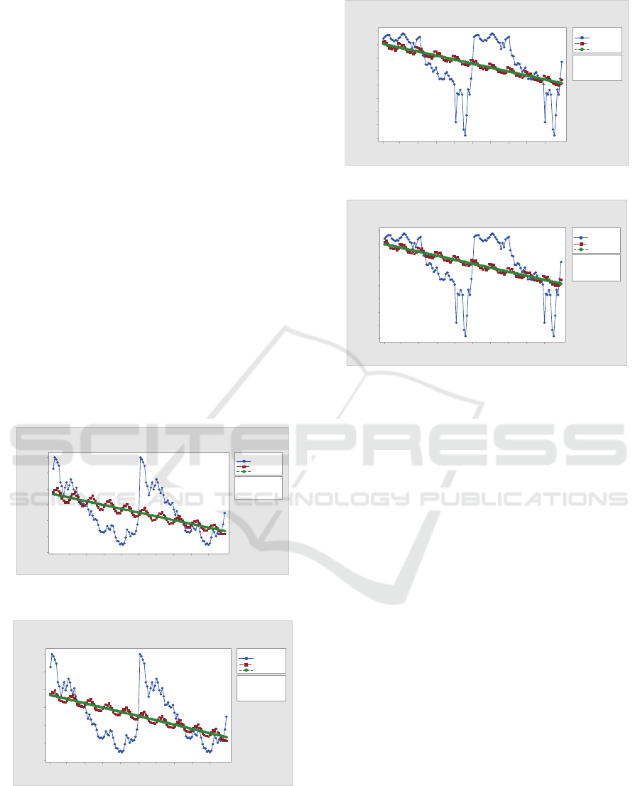
3.4 Decomposition Model
The estimated forecasting models for world
rubber prices using decomposition approach are
presented in Figure 3 (a) and (b) for multiplicative
and additive respectively. Examining these figures,
additive and multiplicative methods are likely to
produce the same pattern and results. Both models
also have a similar trend, namely, a downward trend
with a comparable slope. By examining these
results, both methods can be used to estimate the
same level of accuracy. This conclusion is also
supported by identical MAPE and MAD values (see
Table 3). The MAPE values for both decomposition
forecasting models are 26%, and the MAD values
for both models are 540 and 539. This result
concludes that it is multiplicatively more accurate
than the additive in forecasting world rubber prices.
However, looking at the MSD value, multiplicative
has a smaller MSD value than additives. The MSD
value of the multiplicative decomposition model is
433,526 while the additive MSD value is 436,576.
This unconvincing result implies that forecasters can
use additives or multiplicative to forecast world
rubber prices.
10896847260483624121
4000
3500
3000
2500
2000
1500
1000
MAP E 26
MAD 540
MSD 433526
Accuracy Measures
Index
Wor l d Pr i ce
Actual
Fits
Trend
Variabl e
Time Series Decomposition Plot for World Price
Multiplicative Model
(a) Multiplicative Model
10896847260483624121
4000
3500
3000
2500
2000
1500
1000
MAPE 26
MAD 539
MSD 436576
Accuracy Measures
Index
World Price
Actual
Fits
Trend
Variabl e
Time Series Decomposition Plot for World Price
Additive Model
(b) Additive Model
10896847260483624121
8500
8000
7500
7000
6500
6000
5500
5000
4500
MAPE 10
MAD 675
MSD 725984
Accuracy Measures
Index
Domestic Price
Actual
Fits
Trend
Vari able
Time Series Decomposition Plot for Domestic Price
Multiplicative Model
(c) Multiplicative Model
10896847260483624121
8500
8000
7500
7000
6500
6000
5500
5000
4500
MAPE 10
MAD 676
MSD 725270
Accuracy Measures
Index
Domestic Price
Actual
Fits
Trend
Vari able
Time Series Decomposition Plot for Domestic Price
Additive Model
(d) Additive Model
Figure 3: Decomposition Model for domestic and World
Price
The unconvincing results are also indicated by
the multiplicative and additive decomposition
models for domestic rubber prices as presented in
Figure 3 (c) and (d) as well as Table 3. Figure 3(c)
and (d) also show that additive and multiplicative
likely have similar in pattern and accuracy.
Decomposition plots tend to have downward trends
and similar cyclical patterns. Both additive and
multiplicative decomposition seemingly have a
similar slope. These results imply that the two
forecasting models have the same level of
forecasting accuracy. This means that these two
decomposition models will produce nearly similar
results. This conclusion is more convincing when
viewed from the accuracy of measurement
forecasting, namely, MAPE and MAD (Table 3).
MAPE values for both additive and multiplicative
are the same, i.e., 10%. Looking at MAD,
multiplicative has the lower MSD value than
additive, i.e., 675 and 676 for multiplicative and
additive correspondingly. In addition, based on
MSD value, the multiplicative decomposition model
is less accurate than additive since multiplicative has
a higher value than additive. This means that
forecasters are better off applying an additive
decomposition model to estimate future Indonesian
IRCEB 2018 - 2nd INTERNATIONAL RESEARCH CONFERENCE ON ECONOMICS AND BUSINESS 2018
176
rubber prices. By examining all accuracy measures
used in this research, forecasters can apply an
additive or multiplicative decomposition model for
predicting domestic rubber prices due to
inconclusive result.
Table 3: Accuracy for Forecasting of World and Domestic
Rubber Prices using Decomposition Model
Decomposition
Type
MAPE
(%)
MAD MSD
World
Prices
Additive 26 539 436,576
Multi-
plicative
26 540 433,526
Conclu-
sion
Incon-
clusive
Additive Multipli-
cative
Domes
tic
Prices
Additive 10 676 725,270
Multi-
plicative
10 675 725,984
Conclu-
sion
Incon-
clusive
Multipli-
cative
Additive
151413121110987654321
1.0
0.8
0.6
0.4
0.2
0.0
-0.2
-0.4
-0.6
-0.8
-1.0
Lag
Autocorrelation
Autocorrelation Function for World Price
(with 5% significance limits for the autocorrelations)
(a) World Market
151413121110987654321
1.0
0.8
0.6
0.4
0.2
0.0
-0.2
-0.4
-0.6
-0.8
-1.0
Lag
Autocorrelation
Autocorrelation Function for Domestic Price
(with 5% significance limits for the autocorrelations)
(b) Domestic Markets
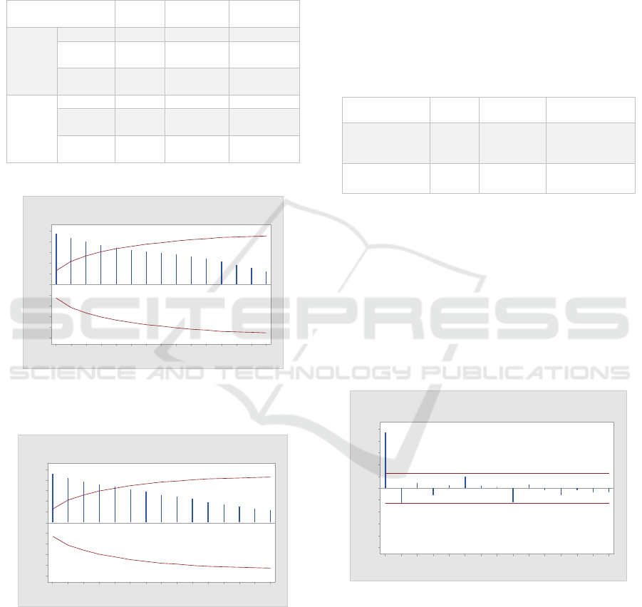
Figure 4: Autocorrelation Function (ACF) for World Price
and Domestic Price
3.5 ARIMA
Stationary test Autoregressive Integrated Moving
Average (ARIMA) is used to complete the monthly
price time series for 5 years. The use of time series
cannot be separated from the problems of
autocorrelation and partial autocorrelation
calculations as illustrated in Figures 4 and 5.
ACF and PACF in Figures 4 and 5 show that the
series is not stationary because the ACF chart does
not die down even though in the PACF there is 1 lag
that is cut off. So, the series needs to be
differentiated. This differentiation is performed with
the Augmented Dickey-Fuller (ADF)
Table 4: Unit Root test with Augmented Dickey-Fuller
(ADF)
Data t-statistic Probability Conclusion
W
orld Market
P
rice
1.648 0.45
2
N
ot Stationary *
)
D
omestic
M
arket Price
1.122 0.69
9
N
ot Stationary *
)
*) is corrected by differencing data accordingly.
Because both price data are not stationary, they
are converted to stationary data on the first
differencing. Then, the ARIMA model for domestic
rubber prices is estimated. After comparing all the fit
statistics, the best model is ARIMA (1,1,4) where all
the parameters are significant at their respective
significance levels (Table 5). Similar steps are also
made for world rubber prices and ARIMA (1,1,4) is
the best model.
151413121110987654321
1.0
0.8
0.6
0.4
0.2
0.0
-0.2
-0.4
-0.6
-0.8
-1.0
Lag
Partial Autocorrelation
Partial Autocorrelation Function for World Price
(with 5% significance limits for the partial autocorrelations)
(a) World Market
Possible Method for Monthly Natural Rubber Price Forecasting
177

151413121110987654321
1.0
0.8
0.6
0.4
0.2
0.0
-0.2
-0.4
-0.6
-0.8
-1.0
Lag
Partial Autocorrelation
Partial Autocorrelation Function for Domestic Price
(with 5% significance limits for the partial autocorrelations)
(b) Domestic Market
Figure 5: Partial Autocorrelation Function (PACF) for
World Price and Domestic Price
Selecting the Possible method for Forecasting
Rubber Prices. Table 6 presents a summary of
accuracy measures for all forecasting models applied
in this research. Among the parametric model used
for world rubber prices, it is very difficult to decide
which is the best forecasting model. If based on
MAPE, ARIMA apparently is the best model with
the lowest value MAPE in which ARIMA generates
5.31 % forecasting error.
However, if based on MAD and MSD, a double
exponential model is the most accurate forecasting
model. This model has the lowest value of MAD
and MSD compared to other models. By following
closely Bowerman et al. (2004); and Hyndman and
Koehler (2006) to use MAPE for reasons of
simplicity, the possible forecasting model for world
rubber price is ARIMA.
Table 6: MAPE, MAD and MSD Value for each
Forecasting Technique
Forecasting
Model
MAPE
(%)
MAD MSD Best
Model
World Price of Rubber
Double
Exponential
Smoothing
5,90 1.33 29,954.6
ARIMA
ARIMA 5,31 14,51 50,630.0
Decompo-
sition
Additive 26 539 436,576.0
Multiplica-
tive
26 540 433,526.0
Domestic Price of Rubber
Double
Exponential
Smoothing
3.000 210 142,285
Double
Exponen-
tial
Smoothing
ARIMA 3.381 27.162 145,695
Decompo-
sition
Additive 10 676 725,270
Multiplica-
tive
10 675 725,984
For domestic rubber prices, the best forecasting
model is the Double Exponential Smoothing Model.
This conclusion is based on two accuracy measures
used in this paper, namely, MAPE and MSD.
Double Exponential Smoothing model has the
lowest MAPE and MSD value compared to other
models even though this model has a higher value of
MAD compared to ARIMA and Decomposition
models. In order words, forecasters are better to
apply double exponential smoothing model to
predict domestic rubber prices in the future.
4 CONCLUSION
The main purpose of this article is to select the right
model and forecasting model for predicting future
rubber prices, both in the domestic market and the
world market. Three types of forecasting methods
were used for this study, i.e., Double Exponential
Smoothing Method, Classical Decomposition
Method and ARIMA. Forecasting method will be
selected with minimum estimated error, that is
minimum value MAPE, MAD, and also MSD.
Although some decisions are not always unanimous,
it is found that ARIMA and Double Exponential
Smoothing models provide the most accurate
prediction of rubber prices with most accuracy
measures.
This finding also implies that depends only on
one forecasting method usually cannot produce a
reliable result. It is better to apply some
methodologies. The methods successfully used in
such commodities, like the regression analysis and
smoothing techniques, are difficult to apply for other
commodities. Such situations also give a great
opportunity for other methods in which the role of
human judgment and experience are higher. The
result of the forecast also depends on the quality of
the applied data.
REFERENCES
Bowerman, B. L., O’Connell, R. T., and Koehler, A. B.
(2004). Forecasting, time series, and regression: An
applied approach. Belmont, CA7 Thomson
Brooks/Cole.
Box, G. E. P., and Jenkins, G. M., (1976). Time Series
Analysis, revised edition, San Francisco: Holden-Day,
1976
Dennis Bergmann, Declan O’Connor, Andreas Thümmel,
(2015) Seasonal and cyclical behaviour of farm gate
IRCEB 2018 - 2nd INTERNATIONAL RESEARCH CONFERENCE ON ECONOMICS AND BUSINESS 2018
178

milk prices, British Food Journal, 117(12): pp.2899-
2913, https://doi.org/10.1108/BFJ-08-2014-0294
Dieng, Dr. Alioune. (2008). Alternative Forecasting
Techniques for Vegetable Prices in Senegal. Reveu
Senegalaise de Recherches agricoles et
agroclimentaires. 1(3): pp. 5 -10. Retrieved from
www.bameinfopol.info/IMG/pdf/Dieng_MP_1_.pdf
Ekananda, Mahyus. (2014). Analisis Data Time Series
Untuk Penelitian Ekonomi, Manajemen dan
Akuntansi. Edisi Pertama. Mitra Wacana Media.
Jakarta.
Fafchamps, M., (2000). Farmers and price fluctuation in
poor countries. Quat. J. Econ., 15: pp. 1–27.
FAO, IFAD, IMF, OECD, UNCTAD, WFP, the World
Bank, the WTO, IFPRI, the UN HLTF, (2011). Price
Volatility in Food and Agricultural Markets: Policy
Responses. Technical Report. FAO and OECD.
Retrieved from
http://www.oecd.org/agriculture/pricevolatilityinfooda
nd agricultural marketspolicyresponses.htm
Grega, C., (2002). Price stabilization as a factor of
competitiveness of agriculture. J. Agric. Econ., 48: pp.
281–284.
Hyndman, Rob J., and Anne B. Koehler. (2006). Another
look at measures of forecast accuracy. International
Journal of Forecasting. 22: pp.679 – 688.
Jatra, A.P., Darnah, A.N. and Syaripuddin. (2013).
Peramalan Index Harga Konsumen (IHK) Kota
Samarinda dengan Metode Double Exponential
Smoothing dan Brown. Jurnal Eksponential, (Online),
4 (1): pp. 39-46.
Karim, R.M., A. Awala and M. Akher. (2010).
Forecasting of Wheat production in Bangladesh.
Bangladesh J. Agric. Res. 35(1): pp. 17 – 28.
Kirchgassner, G. and Wolters, J. (2007) Introduction to
Modern Time Series Analysis. Springer, Berlin
Heidelberg. pp. 1 – 274.
Kumar, T. Vasanth and D.M. Gowda, (2015). Forecasting
of Price of Maize - by an Application of Exponential
Smoothing. International Journal of Current
Agricultural Research, 3(11): pp. 168-172. November
2015.
Pandey, Nivedita and Upadhyay. K.G., (2016). Different
Price Forecasting Techniques and their Application in
Deregulated Electricity Market: A Comprehensive
Study. Paper presented at International Conference on
Emerging Trends in Electrical, Electronics and
Sustainable Energy Systems (ICETEESES–16).
Peng, Wen-Yi and Ching-Wu Chu. 2009. A comparison
of univariate methods for forecasting container
throughout volumes. Mathematical and Computer
Modelling. 50 (2009): pp. 1045 – 1057.
https://doi.org/10.1016/j.mcm.2009.05.027 Retrieved
from
https://www.sciencedirect.com/science/article/pii/S08
95717709001794.
Purba, F. Hero. K. (2011). Komoditi Karet Indonesia
Dalam Pasar Internasional http: // pphp.deptan.go.
id/disp_informasi_/1/5/54/1185/potensi_dan_perkemb
anga _pasar_dunia.html. Accessed at 12 September
2017.
Rajchakit, Manlika. (2017). A New Method for
Forecasting via Feedback Control Theory.
Proceedings of the International MultiConference of
Engineers and Computer Scientists 2017 Vol I,
IMECS 2017, March 15 - 17, 2017, Hong Kong.
Rani, Saima and Irum Raza. (2012). Comparison of Trend
Analysis and Double Exponential Smoothing Methods
for Price Estimation of Major Pulses in Pakistan.
Pakistan J. Agric. Res. 25(3): pp. 234 – 239.
Ribeiro, Celma de Oliveira, Anna Andrea Kajdacsy Balla
Sosnoski and Sydnei Marssal de Oliveira. 2010. Um
modelo hierárquico para previsão de preços de
commodities agrícolas (A Hierarchical Model To
Agricultural Commodities Prices Forecast). Revista
Produção On-line, 10(4): pp. 719 – 733. Accessed:
July 21, 2018. doi:10.14488/1676-1901.v10i4.225.
Robert, R. A., and F.A. Amir, (2009). A New Bayesian
Formulation for Holt's Exponential Smoothing.
Journal of Forecasting, 28: pp. 218–234.
Saini, Deepak, Akash Saxena, and S.L.Surana. (2017).
Hybrid Approach of Additive and Multiplicative
Decomposition Method for Electricity Price
Forecasting. SKIT Research Journal. 7 (1): pp. 12 –
30.
Sudha, CH.K., Rao, V.S and Suresh, CH. (2013). Growth
trends of maize crop in Guntur district of Andhra
Pradesh. International Journal of Agricultural
Statistical Sciences. 9 (1): pp. 215-220.
Sukiyono Ketut, Indra Cahyadinata, Agus Purwoko, Septri
Widiono, Eko Sumartono, Nyayu Neti Asriani, and
Gita Mulyasari. (2017). Assessing Smallholder
Household Vulnerability to Price Volatility of Palm
Fresh Fruit Bunch in Bengkulu Province. International
Journal of Applied Business and Economic Research.
15(3): pp. 1 – 15.
Sukiyono, Ketut and Rosdiana (2018). Pendugaan Model
Peramalan Harga Beras Pada Tingkat Grosir. Jurnal
AGRISEP. 17(1): pp 23 – 30. Maret 2018. DOI:
10.31186/jagrisep.17.1.23-30
Taru, V.B., and M.S.I. Mshelia, (2009). Estimation of
seasonal price variation and price decomposition of
maize and guinea corn in Michika local government
area of Adamawa state. J. Agric. Soc. Sci., 5: pp. 1–6.
Possible Method for Monthly Natural Rubber Price Forecasting
179
