
Forecasting Rainfall at Surabaya using Vector Autoregressive (VAR)
Kalman Filter Method
Yuniar Farida and Luluk Wulandari
Department of Mathematics, Science and Technology Faculty, UIN Sunan Ampel Surabaya
Keywords: Rainfall Forecasting, VAR, VAR – Kalman Filter.
Abstract: Knowing the information of future rainfall data is necessary to increase awareness of the negative impacts of
things caused by rainfall with high intensity to avoid loss and disaster. The aims of this research are forecasting
rainfall at Surabaya city using Vector Autoregressive (VAR). This method is very simple because it is
unnecessary to differentiate between variable of the dependent and independent. VAR is usually applied to
the economic case and has optimal forecasting. But in this research will be applied to the weather case such
as rainfall, humidity, temperature, and wind speed. The model used is the VAR (3) model. From the model,
it is known that the value of R Square of rainfall is 0.56845. It shows that 56.845% model is influenced by
the variable that defined in the model, the rest is influenced by other variables outside the model. Then
obtained the forecast error of rainfall based on the MAPE value is 0.634581019. It shows that the residual
value is high enough so that it needs to be improved using the Kalman Filter method. By applying Kalman
Filter, it has decreased residual value very much. The MAPE value is become 0.008429293. So, the novelty
of this research is VAR – Kalman Filter is very optimal to forecast weather such as rainfall, humidity,
temperature, and wind speed which has fluctuative change.
1 INTRODUCTION
Surabaya is the capital of East Java which is the
second largest city after Jakarta, Indonesia. Total of
population that continues to increase every year,
resulting in the green land of the Surabaya city
decreases every time. Along with the development
and growth of the Surabaya city which continues to
increase every year, causing the change of land
utilization. This has caused continuous reduction of
water infiltration areas since most built as residential
areas. This is a problem for the Surabaya city, because
when the rainy season arrives, Surabaya will occur a
flood.
On December 2014, the floods have occurred in
Surabaya, with reaches a height of up to 15-25 cm
(Fajerial, 2014). On March 2016, there was a flood to
reach a height of up to 50 cm (Ardiansyah, 2016). On
November 2017, floods in Surabaya reached a height
of up to 12,4 cm (ITS Media Center, 2017). Then, on
March 2018, Citraland Surabaya elite housing was hit
by floods again (Abidin, 2018) and there are many
other floods that occurred in Surabaya.
Information on rainfall data is needed in the field
of transportation and agriculture too. In the field of
agriculture, forecasting the amount of rainfall can be
used to determine the dry or rainy season. This
rainfall forecasting will help deal with emerging
problems such as shortages or drought of water. So, it
can reduce the occurrence of crop failure for the
people of western Surabaya in particular. In the field
of transportation, the rainfall data is needed to help
know the weather conditions to support in the process
of transportation activities.
Generally, the benefits of knowing rainfall data
information is needed to increase awareness of the
negative impacts of rainfall that can be caused by high
intensity so that it can avoid loss and disaster. Based
on above explanation, the systematic forecasting of
rainfall time series data needs to show the future
conditions.
Basically, high humidity causes high rainfall. In
addition, the air pressure that is the controlling
element of the climate acts as a factor of the spread of
rainfall. The air pressure will cause the wind and
direction, so it will cause the changes in rainfall and
air temperature (Pradipta, 2013). So, in this research
using variable of wind, humidity and temperature to
predict rainfall in the future. The rainfall data in 2016
can be shown at Figure 1 below:
342
Farida, Y. and Wulandari, L.
Forecasting Rainfall at Surabaya using Vector Autoregressive (VAR) Kalman Filter Method.
DOI: 10.5220/0008521703420349
In Proceedings of the International Conference on Mathematics and Islam (ICMIs 2018), pages 342-349
ISBN: 978-989-758-407-7
Copyright
c
2020 by SCITEPRESS – Science and Technology Publications, Lda. All rights reserved
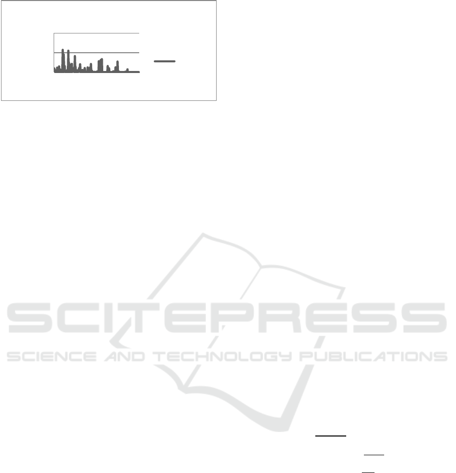
Figure 1: Graph of rainfall data in 2016.
From fig. 1, it shown that rainfall data has a
fluctuative change. It makes rainfall forecasting is
difficult to do. Thus, in this research try to apply a
multivariate forecasting model. The multivariate time
series model is appropriately used if the observed
variable as well as the predicted more than one
(Suharsono, Aziza, & Pramesti, 2017). One of
method for multivariate forecasting model is the
Vector Autogression (VAR). This method is very
simple because it is not necessary to differentiate
between variable of the dependent and independent.
In addition, this method has better estimation results
when compared to other more complicated methods.
(Wei, 2006).
Some studies related to the application of the
VAR model. Analysis time series using VAR model
of wind speeds in Bangui Bay and selected weather
variables in Laoag city, Philippines (Orpia, Mapa, &
Orpia, 2014). Analysis of rainfall and groundwater
using VAR (Chai Yoke Keng1, Shimizu, Imoto,
Lateh, & Peng, 2017), the optimal model is VAR(8)
with all estimated groundwater level values are within
the confidence interval indicating that the model is
reliable. Forecast and isohyet mapping using VAR
model in Semarang (Nugroho, Subanar, Hartati, &
Mustofa, 2014), VAR (6) model is optimal to be
applied with relatively small MAPE and MAE values.
(below 10%). But on the other research about rainfall,
it obtained high error, such as Forecasting rainfall of
Bogor city using VAR (Rosita, Zaekhan, &
Estuningsih, 2018), it obtained 42.18% of MAPE
value.
From related research above, it is known that
VAR model sometimes does not give a good
forecasting result, especially in case of fluctuative
change such as forecasting rainfall. An advanced
method is needed to optimize the forecast results.
Therefore, this research using Kalman Filter method
to estimate the improvement of rainfall forecasting
result of VAR model.
2 THEORITICAL FRAMEWORK
2.1 Stationary Test
The concept often used for stationary testing of time
series data is the unit root test. If a time series data is
non-stationary, then the data contains the unit root
problem. The existence of the root of this unit can be
seen by comparing the value of t-statistics obtained
from the results of predictions with the values of the
Augmented Dickey Fauler test. The equation model
is as follows:
(1)
With
,
length of time lag and . If the root test
of the time series data that is observed is not
stationary, then differencing data. The differencing
model is as follows:
(2)
If the value of δ = 1 is then the variable
is
to be stationary at first degree or symbolized by
and so on.
2.2 Lag Optimal
Identify the optimum order of the model model
using final prediction error (FPE), Akaike’s
Information Criterion (AIC) and Hannan-Quinn
Criterion (HQ) that formulated as follows:
(3)
(4)
(5)
With T is the amount data, K is the amount
variable and
is an MLE estimator from
. Order estimate (̂) of the selected model is
Then, the criteria value of and
that smallest result (Lutkepohl, 2005).
2.3 Johansen Cointegration Test
This cointegration test is to determine the existence
of relationships between variables in the long run. If
there is cointegration on the variables used, then there
is a long-term relationship between variables. The
0
100
200
1
45
89
133
177
221
rainfall data
Rainfall Data
Series1
Forecasting Rainfall at Surabaya using Vector Autoregressive (VAR) Kalman Filter Method
343

usual method used by Johansen cointegration
(Sulistiana, Hidayati, & Sumar, 2017).The Johansen
test is based on the idea of an ADF test on a single
equation obtained from the VAR equation. The VAR
model (2) modified with the ADF process in each
equation is as follows:
(6)
(7)
(8)
2.4 Granger Causality Test
A time series X data has a causal relationship with
time series Y data if by entering the value X before it
can increase the prediction of the value of Y. The
Granger causality model equation that describes the
relationship between X and Y can be written as
follows:
(9)
(10)
2.5 Vector Autoregressive (VAR)
The VAR model was first introduced by Christopher
A. Sims in 1980 applied as a macro economic
analysis (Sulistiana, Hidayati, & Sumar, 2017). The
VAR model is a system of equations that shows all
components of the variable into a linear function of a
constant and the lag values obtained from the
variables present in the system (Shcochrul, 2011).
The general form of the VAR model
denoted , with the following equation:
(11)
or
(12)
which :
= Y vector at time t of the endogenous variable
= a constant value (vector intercept)
= matrix of the value of parameter to
= vector of exogenous variables
= residual residual vector at time
2.6 Kalman Filter
Kalman Filter is one of the very optimal estimation
methods. Transition and measurement equations are
the basic components of applying the Kalman Filter
method. Improved estimation results are based on
measurement data. Estimated polynomial coefficients
and
with the following model equation:
(13)
In this estimate will take the value n = 2. So, equation
(13) changes to :
(14)
With :
and
,
(15)
Which :
= Matrix system
= Input value of iterasi
= Covariance Matrix
= Covariance Matrix R
= Initial value of input
= Initial value of input
Find for values from noise with random ones
normal distribution.
System model :
(16)
(17)
Measurement model :
(18)
(19)
Forecasting step :
Estimation value :
(20)
Covariance value :
(21)
ICMIs 2018 - International Conference on Mathematics and Islam
344
Correction step :
Kalman gain value :
(22)
With and to get correction value from
and
using the formulation as follow :
=
(23)
Final forecasting value :
(24)
which :
= The system state variable at time k whose initial
estimated value is
and the initial covariance
= deterministic input variable at time k
= noise at measurement with mean equal to zero
and covariance of
= measurement variable
H = measurement matrix
= noise at measurement with mean equal to zero
and covariance
.
3 RESEARCH METHOD
3.1 Data and Research Variable
The data used in this research is secondary data
obtained from the Agency Meteorology and
Geophysics (BMKG) East Java. The data used is
daily data of weather and climate element which
include data of rainfall, humidity, air temperature and
wind of Surabaya.
3.2 Method of Research Analyze
The forecasting method used in this research is
Vector Autoregressive (VAR). Then the result of
forecasting, will be estimated using the Kalman filter
method. The research steps are:
1. Stationary test for all variable that used in this
research
2. Choose the optimal lag determination
3. Johansen’s cointegration test
4. Grenger causality test
5. Estimation parameter of VAR model
6. Verify of var model
7. Forecasting using var model
8. Improved forecasting results using Kalman
Filter.
4 RESULT AND DISCUSSION
Before to the establishment of the VAR model, it is
necessary to show descriptive statistics of the data
used in this research. Descriptive statistics of data are
listed in table 1.
Table 1: Statistics descriptive variable of research.
Temperature
Rainfall
Wind
Humidity
Mean
28,21
0,056
4,958
77,714
Med
28,3
0
5
78
Max
30
1
9
92
Min
26,2
0
2
59
S.
Dev
0,815
0,142
1,469
5,776
4.1 Establishment VAR Model
4.1.1 Stationary Test
A time series data is classified as stationary data if
there are not unit roots in the data sequence (Basuki
& Prawoto, 2016). In this research, used Augmented
Dickey Fuller (ADF) test method to know the
stationary of data. Table 2 is the result of test
stationary data using ADF test method.
Table 2: Results of stationary test ADF.
Variable
ADF (Level)
t- statistic
Critical
Value
MacKinnon
(5%)
Prob*
ADF
Rainfall
-6,500513
-2,87263
0
Humidity
-3,148574
-2,872675
0,024
Wind
-4,655735
-2,87263
0
Temperature
-6,169448
-2,87263
0
A data is classified as stationary if the absolute
value of the ADF statistic t is more than MacKinnon
criterion at the 5% confidence level, otherwise the
significance value of each variable is less than 0.05
(Herlinda, 2013).
From stationary test data using ADF test method,
it is known that all data stationary, so it’s unnecessary
to be differencing again.
Forecasting Rainfall at Surabaya using Vector Autoregressive (VAR) Kalman Filter Method
345
4.1.2 Optimal Lag Determination
Determine the length and the shortness of a lag in the
VAR model is very important. If the lag we use in the
VAR model is too short, then it cannot explain the
dynamics of a model. While if it is too long, it will
result in inefficient model estimation (Basuki &
Prawoto, 2016). Table 3 is the result of optimal lag:
Table 3: Result of optimal lag determination.
Lag
AIC
SC
HQ
0
11,14250
11,19901
11,16524
1
9,592247
9,874774*
9,705969*
2
9,601822
10,11037
9,806520
3
9,535894*
10,27046
9,831570
4
9,572256
10,53285
9,958909
5
9,550203
10,73681
10,02783
Table 3 shows that the AIC value (9.535894) is
smaller than SC (9,874774) and HQ (9.705969).
Since the AIC value in the 3rd lag, it can be concluded
that the optimal lag is 3.
4.1.3 Johansen’s Cointegration Test
Cointegration test is used to determine the balance in
the long time. It's means, there are similarities in
movement and stability of relations between all
variables in the research study or not. In this research
used Johansen's cointegration test method. Table 4
and 5 is the results of the cointegration test.
Table 4: Unrestricted Cointegration Rank Test (Trace).
Eigen
value
Trace
Statistic
Critical
Value
(5%)
Prob
None
0,179
109,606
47,8561
0,0000
At Most 1
0,112
59,1725
29,7971
0,0000
At Most 2
0,085
28,9108
15,4947
0,0003
At Most 3
0,024
6,19839
3,84146
0,0128
Table 5: Unrestricted Cointegration Rank Test (Maximum
Eigen value).
Eigen
value
Max-
Eigen
Statistic
Critical
Value
(5%)
Prob
None
0,1794
50,4333
27,5843
0,0000
At Most
1
0,1119
30,2617
21,1316
0,0020
At Most
2
0,0852
22,7123
14,2616
0,0019
At Most
3
0,024
6,19839
3,84146
0,0128
Statistic test:
H
0
: There isn’t cointegration
H
1
: There is cointegration
H
0
is accepted if Trace statistic and Max Eigen
Statistic is greater than Critical value at the 0.05
confidence level.
Based on the table above, H
0
is accepted. So, it
can be concluded that between one variable and
another doesn’t have stability and balance relation in
long time.
4.1.4 Granger Causality Test
Granger causality test is used to know the relation of
causality among variables one with other variables.
Table 6 is Granger causality test results.
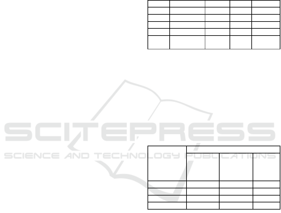
Table 6: Granger causality test results.
Hipotesis Null
Obs
F-
Statistic
P-
value
Wind does not Granger
cause rainfall
256
0,67977
0,565
Rainfall does not
Granger cause wind
1,07136
0,362
Temperature does not
Granger cause rainfall
256
2,67286
0,048
Rainfall does not
Granger cause
temperature
0,15716
0,925
Humidity does not
Granger cause rainfall
256
5,11051
0,002
Rainfall does not
Granger cause humidity
1,91108
0,128
Temperature does not
Granger cause wind
256
0,93967
0,422
Wind does not Granger
cause temperature
1,65428
0,177
Humidity does not
Granger cause wind
256
0,74456
0,526
Wind does not Granger
cause humidity
0,11262
0,953
Humidity does not
Granger cause
temperature
256
2,30037
0,078
Temperature does not
Granger cause humidity
1,25749
0,289
From table 4 above obtained that:
Hypothesis for all variables X (wind, temperature,
humidity) to Y (rainfall)
H
0
= X doesn’t Granger cause of Y
H
1
= X Granger cause of Y
On other side, we find Granger causality for
variabel Y to all of variables X with hypothesis:
H
0
= Y doesn’t Granger cause X
ICMIs 2018 - International Conference on Mathematics and Islam
346
H
1
= Y Granger cause of X
Statistic test:
H
0
is accepted if p-value > α (0,05)
Based on the table above, it is known that only
variables of humidity and temperature Granger cause
of rainfall (humidity and temperature have
unidirectional causality with rainfall)
4.1.5 Estimation Parameter of VAR Model
The next step of this research is estimation parameters
of VAR model. Because the optimal lag is 3 and
consists of 4 variables, so the VAR (3) models are:
(25).
((b...................................................
(26).
(27).
(28).
which:
R = Rainfall
T = Temperature
H = Humidity
W = Wind speed
From the VAR model above, it obtains result R
Square value of 0.56845. It shows that 56.845%
model is influenced by the variable that defined in the
model, the rest is influenced by other variables
outside the model.
4.1.6 Verify the VAR Model
In performing the model verification test, residual
normality test will be performed. Tables 7 is the
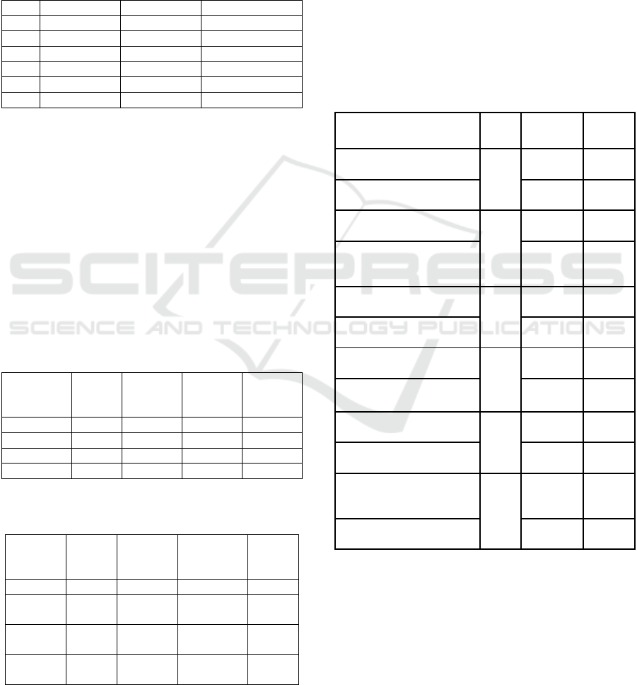
results of residual normality testing.
Table 7: Residual normality test.
Variable
Skewness
Chi-
Square
Df
Prob.
1
3,461298
511,1717
1
0,000
2
0,182689
1,424016
1
0,2327
3
0,564558
13,59896
1
0,0002
4
-0,340428
4,944698
1
0,0262
Joint
531,1394
4
0,0000
Based on residual normality test, it obtained
values of skewness smaller than the critical value of
Chi-Square, it can be concluded that the residual is
normally distributed.
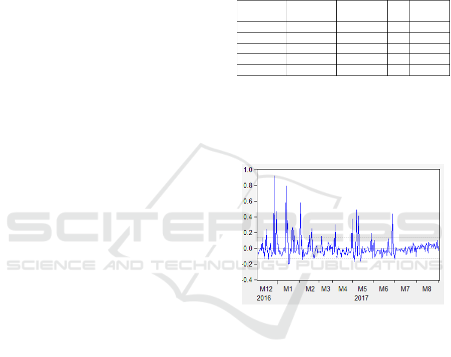
The verification model can also be shown by the
plot of the error as presented in Figure 2.
Figure 2: Graph of rainfall forecasting data error.
In Figure 2 above, the error does not form a certain
pattern and is distributed around zero. So, it can be
concluded that the error has an independent nature.
Thus, the assumption on a good VAR model is used
for forecasting.
4.1.7 Forecasting using VAR Model
The VAR (3) model will be used to obtain future
rainfall forecast for 2 weeks. Table 8 shows the
comparison of actual data with forecasting data and
residual value.
Forecasting Rainfall at Surabaya using Vector Autoregressive (VAR) Kalman Filter Method
347
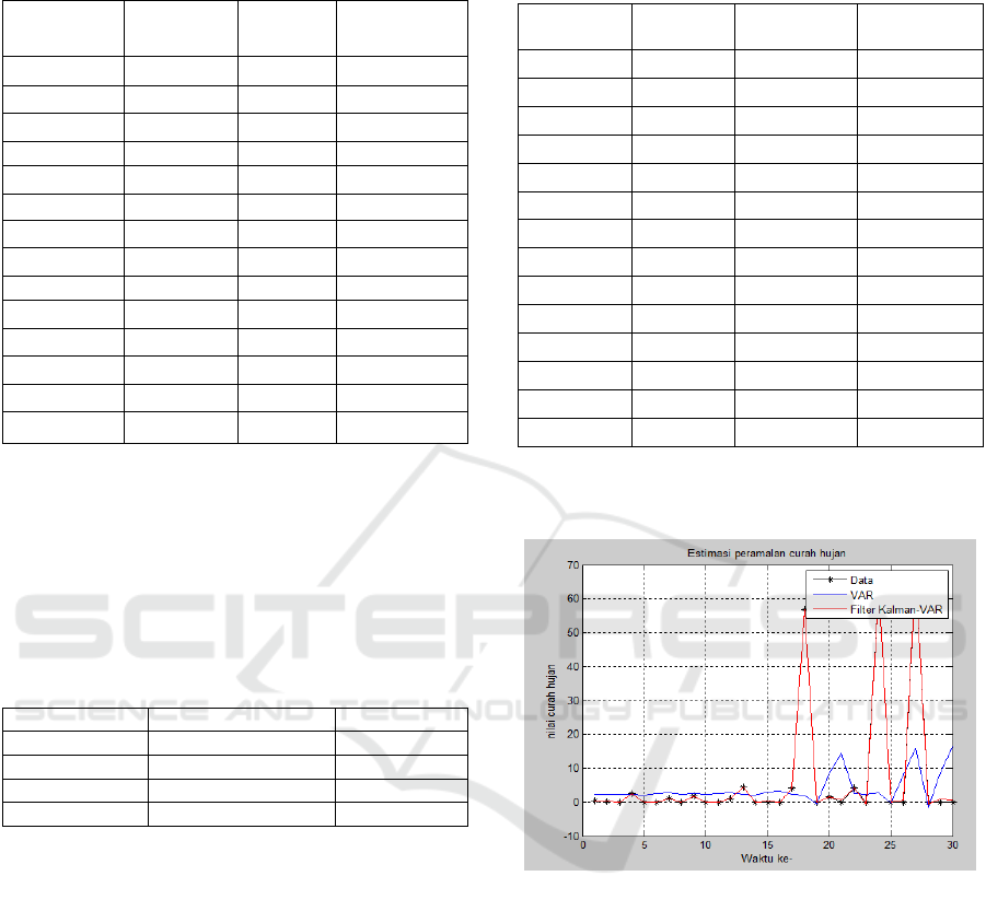
Table 8: Comparison actual data and forecast result of
rainfall.
Date
Actual
(mm)
VAR
Residual
13/04/2017
0,4
2,3539
1,9539
14/04/2017
0,2
2,2473
2,0473
15/04/2017
0
2,3369
2,3369
16/04/2017
2,4
2,3371
0,0629
17/04/2017
0
2,1621
2,1621
18/04/2017
0
2,4528
2,4528
19/04/2017
1,2
2,7984
1,5984
20/04/2017
0
2,1766
2,1766
21/04/2017
1,8
2,4076
0,6076
22/04/2017
0
2,3485
2,3485
23/04/2017
0
2,46
2,46
24/04/2017
1
2,6576
1,6576
25/04/2017
4,3
2,1927
2,1073
26/04/2017
0
2,0989
2,0989
Then, the VAR (3) model can also be used to
obtain future temperature, humidity and wind speed
forecast for 2 weeks.
Forecasting results using VAR (3) obtained the
forecast data with high error. This is indicated by the
MAPE and the R-Square value of each model as in
table 9.
Table 9: MAPE and R-Square value of each model.
Variable
MAPE
R-Square
Rainfall
0,634581019
0,568645
Humidity
0,234174028
0,182294
Temperature
0,185383523
0,244976
Wind speed
0,724709869
0,368949
Thus, in order to handle this, a model is required
to improve the forecast result of VAR model. In this
research, using Kalman Filter method.
4.2 Improved Forecasting Results
using Kalman Filter
Forecasting data using VAR method obtained R-
Square level that small and obtained the big residual
level, it is necessary to improve the forecasting result
using Kalman Filter method. The result of rainfall
forecasting using VAR – Kalman Filter method in
Table 10.
Table 10: Comparison actual data, VAR – KF and Residual
Value of Rainfall.
Date
Actual
(mm)
VAR – KF
Residual
13/04/2017
0,4
0,4834132
0,0834132
14/04/2017
0,2
0,1961469
0,00385306
15/04/2017
0
0,01080127
0,01080127
16/04/2017
2,4
2,40160714
0,00160714
17/04/2017
0
0,00803065
0,00803065
18/04/2017
0
0,02364565
0,02364565
19/04/2017
1,2
1,19956301
0,00043699
20/04/2017
0
0,01173313
0,01173313
21/04/2017
1,8
1,79934212
0,00065787
22/04/2017
0
0,00770355
0,00770355
23/04/2017
0
0,00997199
0,009971998
24/04/2017
1
0,99815334
0,001846656
25/04/2017
4,3
4,30028570
0,000285701
26/04/2017
0
0,01049394
0,010493944
Figure 3 is plot of actual data, VAR and VAR –
Kalman Filter rainfall.
Figure 3: Plot of actual data, VAR and VAR – Kalman
Filter rainfall.
From the plot of data above, it is known that the
result of VAR forecasting after improving with the
Kalman Filter closer to the actual data.
In this research, it is proven that the Kalman Filter
method is very optimal for improving the forecast
result of VAR model. This is indicated with
comparison MAPE for VAR and VAR – Kalman
Filter on each variable as shown in Table 11.
ICMIs 2018 - International Conference on Mathematics and Islam
348

Table 11: Comparison MAPE of VAR and VAR – Kalman
Filter on each variable.
VAR
VAR – KF
Rainfall
0,634581019
0,008429293
Humidity
0,234174028
1,2987E-08
Temperature
0,185383523
3,18158E-08
Wind speed
0,724709869
0,000609279
5 CONCLUSIONS
The model used in forecasting is the VAR (3) model.
With the equation as follows:
+
.....
................................................
+
+
.....................................................
From the model, it is known that the value of R
Square of rainfall is 0.56845. It shows that 56.845%
model is influenced by the variable that defined in the
model, the rest is influenced by other variables
outside the model. Then obtained the forecast error
based on the MAPE value is 0.634581019.
Forecasting rainfall using VAR (3) obtained high
enough residual value, so it is necessary to improve it
using the Kalman Filter method. Improvement VAR
forecasting using Kalman Filter proved to be very
optimal. It has decreased residual value very much.
The MAPE value of rainfall is become 0.008429293.
REFERENCES
Abidin, Z. 2018. Citraland Dikepung Banjir, Tunda Dulu
Malam Minggu Anda. Surabaya: Suarasurabaya.net.
Ardiansyah, M. 2016. Hujan kembali guyur Surabaya,
banjir di mana-mana. Surabaya: Merdeka.com.
Basuki, A. T., & Prawoto, N. 2016. Analisis Regresi dalam
Penelitian Ekonomi & Bisnis: Dilengkapi Aplikasi
SPSS & Eviews. Depok: Rajawali Press.
Chai Yoke Keng1, a. F., Shimizu, K., Imoto, T., Lateh, H.,
& Peng, a. K. 2017. Application of vector
autoregressive model for rainfall and groundwater level
analysis. AIP Conference Proceedings Volume 1870
Issue 1.
Fajerial, E. 2014. Hujan 4 Jam, Pemkot Surabaya: Cuma
Genangan. Surabaya: TEMPO.COM.
Herlinda, T. 2013. Peramalan Polusi Udara Oleh Karbon
Monoksida (CO) Di Kota Pekanbaru Dengan
Menggunakan Model Vector Autoregressive (VAR).
Pekanbaru: Universitas Islam Negeri Sultan Syarif
Kasim Riau.
ITS Media Center. 2017. Intensitas Curah Hujan Penyebab
Surabaya Dikepung Banjir. Surabaya.
Lutkepohl, H. 2005. New Introduction to Multiple Time
Series Analysis. Berlin: Springer.
Nugroho, A., Subanar, Hartati, S., & Mustofa, K. 2014.
Vector Autoregression (Var) Model for Rainfall
Forecast and Isohyet Mapping in Semarang – Central
Java – Indonesia. (IJACSA) International Journal of
Advanced Computer Science and Applications Vol. 5,
No. 11, 44-49.
Orpia, C., Mapa, D. S., & Orpia, J. 2014. Time Series
Analysis using Vector Auto Regressive (VAR) Model
of Wind Speeds in Bangui Bay and Selected Weather
Variables in Laoag City, Philippines. Munich Personal
RePEc Archive.
Pradipta, N. 2013. Analisis Pengaruh Curah Hujan di Kota
Medan. Jurnal: Saintia Matematika 1.
Rosita, T., Zaekhan, & Estuningsih, R. D. 2018. Vector
Autoregressive (VAR) for Rainfall Prediction.
International Journal of Engineering and Management
Research ISSN (ONLINE): 2250-0758, ISSN (PRINT):
2394-6962, 96-102.
Shcochrul, R. A. 2011. Cara Cerdas Menguasai Eviews.
Jakarta: Salemba Empat.
Suharsono, A., Aziza, A., & Pramesti, a. W. 2017.
Comparison of Vector Autoregressive (VAR) and
Vector Error Correction Models (VECM) for Index of
ASEAN Stock Price. International Conference and
Workshop on Mathematical Analysis and its
Applications 978-0-7354-1605-5.
Sulistiana, I., Hidayati, & Sumar. 2017. VAR and VECM
Approach for Inflation Relations Analysis, Gross
Regional Domestic Product (GDP), Word Tin Price, Bi
Rate and Rupiah Exchange Rate. Integrated Journal of
Business and Economics ISSN: 2549-3280.
Wei, W. W. 2006. Time Series Analysis: Univariate and
Multivariate Methods. United State of America:
Addison-Wesley Publishing Company.
Forecasting Rainfall at Surabaya using Vector Autoregressive (VAR) Kalman Filter Method
349
