
Biochemical Oxygen Demand Level Modeling in Surabaya River
using Approach of Cokriging Method
Suliyanto
Department of Mathematics, Universitas Airlangga, Surabaya, Indonesia
Keywords: Surabaya River, BOD, COD, Cokriging Method.
Abstract: National Coordinator of Indowater Community of Practice said that the Surabaya River contains high
pollutants that cause pollution. One of the parameters for estimating pollution of Surabaya River is
Biochemical Oxygen Demand (BOD). In addition to BOD there are other parameters that have a correlation
with BOD, namely Chemical Oxygen Demand (COD). The kriging method is used to estimate the level of
water pollution in a new location based on observational data around it using both parameters. The purpose
of this research is to estimate BOD levels in three locations around the industry using the method of cokriging.
Observation of 10 samples of BOD and COD showed significant correlation for α = 5% with a correlation
value of 99.5% and P-value of 0.000. The result of cross-validation estimation of BOD level sampled using
Gaussian model obtained high R
2
value equal to 91.6% and Root Sum Squared (RSS) value is small, that is
0.7057 so it can be said that interpolation result accurate. The results showed that BOD levels leading
downstream were lower. This is because the source of pollutants from the upstream of the river that leads to
downstream of the river is less affected.
1 INTRODUCTION
According to the monitoring of Jasa Tirta I Public
Company, there are five rivers in East Java that do not
meet the water quality standard, one of which is the
Surabaya River. National Coordinator Indowater
Community of Practice, Riska Darmawanti said that
the Surabaya River contains high pollutants,
evidenced by the level of 420 ng / g plastic samples.
In addition there are also organochlorine pesticides
and detergent waste (Haq, 2017). The result of the
research by pollution index method concluded that
the biggest contaminant contributor in Surabaya
River is phenol and total suspended solids (Priyono et
al., 2013). The pollutant parameters of the Surabaya
River are Biochemical Oxygen Demand (BOD)
(Trisnawati and Masduqi, 2013). Research on the
correlation of Chemical Oxygen Demand (COD) and
BOD of liquid waste for pollution monitoring of
Surabaya River shows that there is a linear correlation
between COD and BOD of Surabaya River water
(Razif and Masduqi, 1996). Calculation statistically
with descriptive analysis obtained the result that BOD
parameter contributes to domestic waste equal to
59.77%, industrial waste 40.05% and agricultural
waste 0.18% while for the parameter of COD
contribute domestic waste equal to 54.11%, industrial
waste 45.74% and agricultural waste 0.15% (Suwari,
2010). The result of measurement by Surabaya
Environment Department (ED) 2016, BOD level at
the sample location does not meet the standard quality
of class II water quality that has been established. The
role of BOD and COD is equivalent to other
parameters that are key parameters in relation to
alleged pollution by certain activities (Atima, 2014).
BOD measurements require a five-day long-term cost
and time analysis with complex processes because it
takes highly acclimatized and active bacteria seeds in
high concentrations (Tchobanoglous, 1991). The
measurement of BOD in the Surabaya River
undertaken by ED Surabaya is still limited to a few
points. One effort to minimize the time and cost of
measuring BOD in the Surabaya River is the point
estimation method.
Geostatistics is defined as a method that discusses
the spatial relationships of several variables to
estimate the value of variables located in unobserved
locations (Kelkar and Perez, 2002). The appropriate
method for use in the data of the sampled BOD level
consisting of only one variable is kriging. In fact, the
parameters of water pollution in rivers are not only
BOD but also COD. Another method that can be used
52
Suliyanto, .
Biochemical Oxygen Demand Level Modeling in Surabaya River using Approach of Cokriging Method.
DOI: 10.5220/0008517100520059
In Proceedings of the International Conference on Mathematics and Islam (ICMIs 2018), pages 52-59
ISBN: 978-989-758-407-7
Copyright
c
2020 by SCITEPRESS – Science and Technology Publications, Lda. All rights reserved

to solve this case is the cokriging method with
attention to other water pollution parameters that is
COD to calculate BOD level. BOD is chosen as the
primary variable because it is one of the important
parameters related to wastewater treatment
(Tchobanoglous, 1991). While COD is chosen as a
secondary variable because the measurement time is
shorter, only for one to two hours only. In addition,
COD has also included the level in BOD because
COD is a total picture of organic matter while BOD
is a description of organic material that easily
explained only (Tchobanoglous, 1991). Therefore,
BOD can be predicted with COD, but COD may not
be suspected by BOD because BOD cannot describe
the total organic matter in the waters.
Research using browning method on river
pollution case has never been done. Some research
using kriging and cokriging method has been done by
Ahmadi and Sedghamiz (2008) using kriging and
cokriging method in its application to groundwater
depth mapping. The results showed that both methods
were acceptable but based on the Mean Square Error
(MSE)value, the cokriging method gave more
accurate results in mapping the depth of groundwater
throughout the study area. Based on the description,
the researcher is interested to apply the cokriging
method to estimate BOD concentration based on
COD concentration observed by ED of Surabaya city,
to know BOD concentration at unobserved point
specially at points close to industrial or factory that
discharges its waste to channel on the Surabaya River
as a pollution measure of the Surabaya River.
2 METHODS
2.1 Stationary
Geostatistical data can be analyzed using kriging or
cokriging method if it has qualified stationary. The
stationary assumptions must be met both stationary in
the mean (stationarity of order one) and stationary
invariance (second order stationery). According to
Kelkar (2002), the first order stationarity can be
written mathematically as follows:
(1)
With
is variable Z at location .
For the second-order stationarity can be written
mathematically as follows:
. (2)
Covariance in a stationary region is a function of only
the vector h, not of the variable itself. That means that
as long as the distance and the direction between two
points can be predicted the covariance between
random variables at two points. No random variable
is needed in that location. Therefore, equation (2) can
be written as follows:
, (3)
where
is covariance at distance.
2.2 Spatial Relationships
The most common spatial relationships used in
geostatistics are covariance, correlation and
variogram.
2.2.1 Covariance
Equations (1) and (2) explain covariance under the
assumption of stationarity of order one and two. The
covariance of the z variable at location and the
variable z at the location of is
. (4)
2.2.2 Correlation Coefficient
The correlation coefficient used to describe the spatial
relationship. From equation (4) is defined correlation
coefficient as follows
, (5)
where
is covariance at distance ,
is the
standard deviation of data at location . If a second-
order stationary assumption is used, then it is obtained
. (6)
From equation (6) is obtained
(7)
The substitution of (7) to (5) is obtained
. (8)
The correlation coefficient at (8) is estimated from the
sample as follows:
Biochemical Oxygen Demand Level Modeling in Surabaya River using Approach of Cokriging Method
53

, (9)
with is the sample variance.
2.2.3 Variogram
Variogram is a measure of data variance that takes
into account distance. A variogram () is one of the
basic geostatistical tools that is used to determine
spatial dependence. It is often referred to as a
semivariogram (), which has exactly the same
characteristics (Kis, 2016). According to Kelkar
(2002) semivariogram is defined as follows:
, (10)
with γ(h) is a semivariogram or semivariance at a
distance h. Based on the definition of the variance of
equation (10) can be written as follows:
(11)
Substitutions (3) and (6) to (11) are obtained
(12)
There are two types of variograms: experimental
variogram and theoretical variogram. According to
Kelkar (2002) calculate the value of the experimental
variogram as follows:
, (13)
with
is the semivariance estimate based on the
sample data at distance. Meanwhile, to calculate
variogram that there is a cross-link or commonly
referred to as cross variance can be written as follows:
(14)
The estimation of cross variance between variables z
and z2 at (14) is
(15)
The cross covariance equation is
(16)
The cross-covariance estimation between the z and z2
variables at (16) is
(17)
According to Isaaks and Srivastava (1989), there
are several components in the variogram of sill,
nugget, and range. Sill (
) is the value of the
variogram in the upper part of the variogram (level
off), can also be interpreted as the "amplitude" of a
particular component of the variogram. Range (
) is
the distance at which the variogram reaches the sill.
In theory, the initial value of the variogram is zero.
When the lag approaches zero the value of the
variogram is referred to as the nugget. The nugget
(
) represents a variation in the very small distance
(lag), including error in measurement.
2.2.4 Theoretical Variogram
The theoretical variogram is a variogram that is
arranged by function or has a curve shape close to the
experimental variogram. For further analytical
purposes, the experimental variogram should be
replaced by the theoretical variogram. This
substitution aims to model the variogram according to
the characteristics of the estimated variables. There
are two types of theoretical variogram: isotropic
variogram and anisotropic. According to LeMay
(1995) variogram which depends only on distance
and point on the direction called isotropy variogram.
According to Kelkar (2002), there are four models of
the isotropic variogram, i.e., linear, spherical,
exponential, and Gaussian models. The isotropic
variogram equation for linear model (figure 1) is
. (17.a)
The isotropic variogram equation for spherical model
(figure 2) is
(17.b)
With
is a spherical model at a distance of
. The corresponding covariance equation is
ICMIs 2018 - International Conference on Mathematics and Islam
54
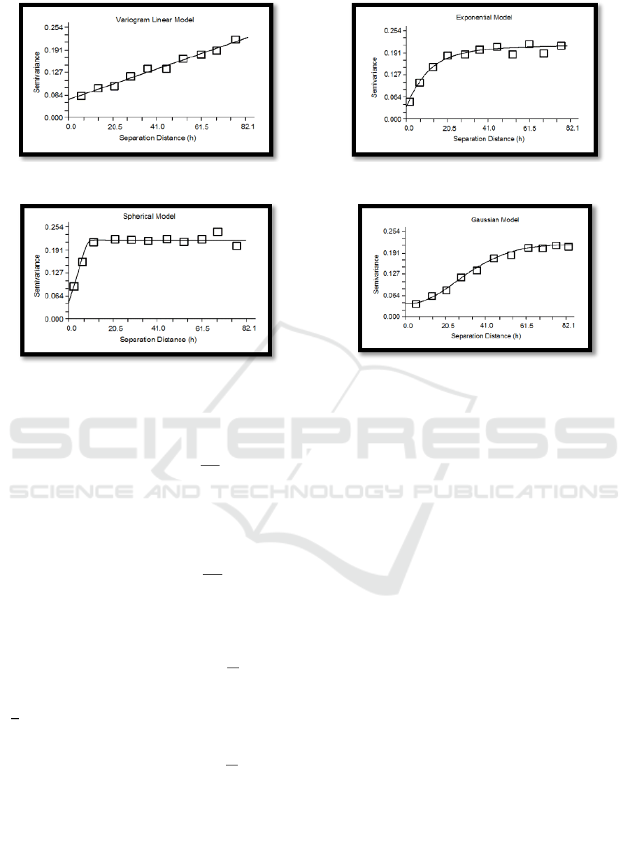
Figure 1: Theoretical Variogram of Linear Model.
Figure 2: Theoretical Variogram of Spherical Model.
Theisotropic variogram equation for exponential
model is
(17.c)
with
is an exponential model at a distance of
. The corresponding covariance equation
(figure 3) is
.
The isotropic variogram equation for gaussian model
(figure 4) is
, (17.d)
with
is a gaussian model at a distance of
. The corresponding covariance equation is
.
Figure 3: Theoretical Variogram of Exponential Model.
Figure 4: Theoretical Variogram of Gaussian Model.
Root Sum Squared (RSS) validation information is
used to determine the variogram model match. The
best isotropic theoretical variogram model is the
model with the smallest RSS value.
2.3 Cokriging Method
The cokriging method is the interpolation method
used to estimate the level of a variable with respect to
other variables (Isaaks and Srivastava 1989). The
estimation equation of cokriging according to Kelkar
(2002) is
(18)
with
is the estimated value at the new location,
is the browning weighter for variable Z at the alleged
location,
is the brown weighing for the variable Z,
is the brown weighing variable Z2,
is the
value of variable Z at location ,
is the value of
variable Z2 at location
2.3.1 Unbiased Condition
If
is the value of a variable in a new location that
is not sampled it will be estimated, then
is an
unbiased estimator for
which satisfies the
following equation
Biochemical Oxygen Demand Level Modeling in Surabaya River using Approach of Cokriging Method
55

(19)
Substitutions (18) to (19) are obtained
(20)
From (20) under the assumption of a first-order
stationer is obtained
(21)
From (21) obtained
. (22)
The value of
at (22) is considered 0 to be obtained
. (23)
Two constraints within (23) produce an ordinary
cokriging system. If (23) is substituted to (22), then
is obtained, so that from equation (18) is
obtained the estimated variable in the new location as
follows
. (24)
2.3.2 Minimum Variance
The estimation of the cokriging equation (24) is
obtained by minimizing the variance as follows:
. (25)
with constraints (23). Parameter estimation of the
cokriging model (24)uses the Lagrange multiplier
method by minimizing function as follows:
(26)
3 RESULTS AND DISCUSSION
The data used in this research are BOD and COD
concentration at ten location points in Surabaya River
in 2016. Before estimating the level of river pollution
using BOD level at a new location or location to be
expected, it is necessary to validate by estimating the
observation data which has been obtained.
3.1 Validation of BOD Level
Before estimating the level of river pollution using
BOD level at a new location to be expected, it is
necessary to validate it first by estimating the
observed data that has been obtained. It is assumed
that BOD and COD level data satisfy stationary
assumptions in mean and variance.
The parson correlation value between BOD and
COD shows p-value equal to 0,000 which means
significant at α = 5%. The correlation value between
BOD and COD variables is 99.5%. The cokriging
method can be continued because BOD and COD
variables have a high correlation. Variogram used in
this research is theoretical isotropic variogram
consisting of four models, namely linear, spherical,
exponential, and Gaussian model. Isotropic
variogram depends only on distance () alone without
considering direction. Variogram and cross-
variogram theoretical selected to determine the
suitability of the model based on the smallest
Residual Sum of Square (RSS) value. The result of
modeling theoretical isotropy variogram from BOD
and COD levels for the four models is presented in
the following table 1.
Based on Table 1 obtained the best theoretical
variogram model for BOD is the Gaussian model with
the smallest RSS value of 2838. In this model, BOD
level reaches sill in the range of 2050 meters which
means the BOD level will not have any dependencies
at distances over 2050 meters. Based on the nugget-
sill ratio of theoretical isotropic variograms, BOD
levels are included in strong spatial autocorrelation of
0.408%. The best theoretical variogram model for
COD is the Gaussian model with the smallest RSS
value of 144803. In this model, the COD level reaches
sill at 2100 meters range which means COD level will
not have dependencies more than 2100 meters. Based
on the nugget-sill ratio of theoretical isotropic
variograms, COD levels are included in strong spatial
autocorrelation of 0.312%. The best theoretical
variogram model for cross-variogram of BOD and
COD is the Gaussian model with the smallest RSS
value of 20297. In the selected model for cross
variogram, there is a dependency between BOD and
COD level at 2090 meters distances, more than 2090
meters no dependencies between both. The best
theoretical isotropic variogram model for BOD level
is presented in the following figure 5.
Figure 6 is the best theoretical isotropic variogram
model of COD level. While the best theoretical
isotropic cross-variogram model of BOD and COD
levels as Figure 7.
ICMIs 2018 - International Conference on Mathematics and Islam
56
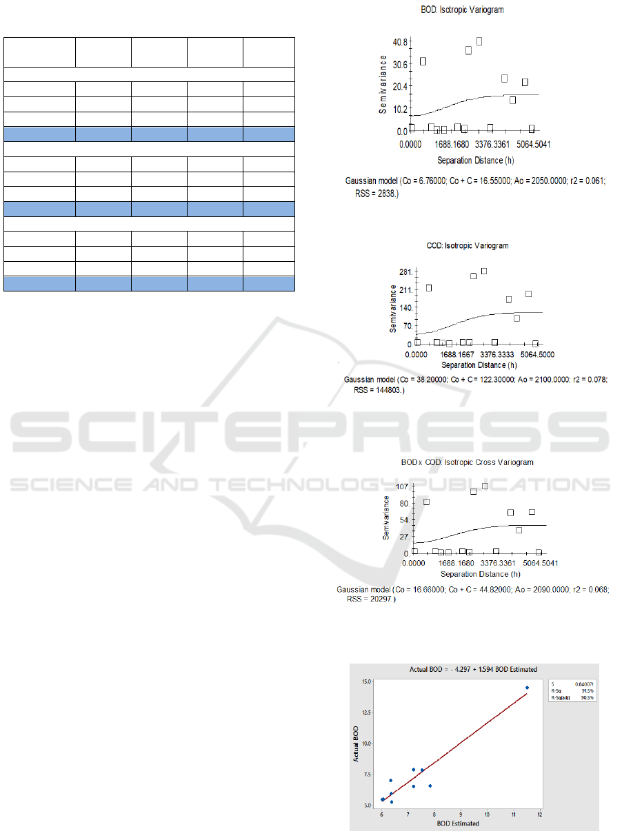
Table 1: Parameter Estimation Result of Cokriging Model
on BOD and COD Data.
Model
Nugget
(C
o
)
Sill
(C
o
+C)
Range
(A
0
)
RSS
BOD
Linear
8.508
17.05
4987.5
2925
Spherical
5.280
15.88
3580.0
2846
Exponential
6.050
17.33
6420.0
2887
Gaussian
6.760
16.55
2050.0
2838
COD
Linear
51.879
128.34
4987.5
149374
Spherical
31.500
117.30
3940.0
145603
Exponential
29.300
126.80
6150.0
147688
Gaussian
38.200
122.30
2100.0
144803
BOD x COD
Linear
21.037
46.58
4987.5
20936
Spherical
12.860
43.02
3770.0
20382
Exponential
14.700
48.50
7170.0
20679
Gaussian
16.660
44.82
2090.0
20297
3.2 Cokriging Interpolation to
Estimate the BOD Level
After the best theoretical variogram and theoretical
cross-variogram are obtained, then it is used for
cokriging interpolation. The purpose of cokriging
interpolation is to estimate BOD and COD levels
using point estimation because the coverage of
measurement region is not broad, i.e. in one river
zone. Based on the actual value and estimated value
of brown interpolation result, then cross-validation is
done to see the good of the interpolation result. The
effect of cross-validation obtained by coefficient of
determination
value of 91.5% as presented as
figure 8.
Mean Square Error (MSE) value of 0.7057. The
value of
is very high, and the MSE value is small,
so the interpolation result is accurate. The accuracy of
BOD value estimation can also be seen through the
plot between the actual value and the estimated value
of BOD level as figure 9.
3.3 BOD Estimated on New Location
The estimated spread of BOD levels in the Surabaya
River is presented in the form of a two-dimensional
contour map (figure 10).
The cokriging interpolation results in a range of
BOD levels which vary between 6 mg / l to 11.7 mg / l
which are grouped into 15 intervals in the form of
different color gradations. The area marked by the
symbol X is the measurement point for BOD levels in
the Surabaya River by ED. The estimated BOD content
is dominated at intervals of 7.1 mg / l to 7.5 mg / l
which are indicated by gradations of light green.
Figure 5: Best Theoretical Isotropic Variogram of BOD
level.
Figure 6: Best Theoretical Isotropic Variogram of COD
level.
Figure 7: Best Theoretical Isotropic Cross Variogram of
BOD and COD levels.
Figure 8: Cross-Validation of BOD Level Estimates at the
Observation Locations.
Biochemical Oxygen Demand Level Modeling in Surabaya River using Approach of Cokriging Method
57
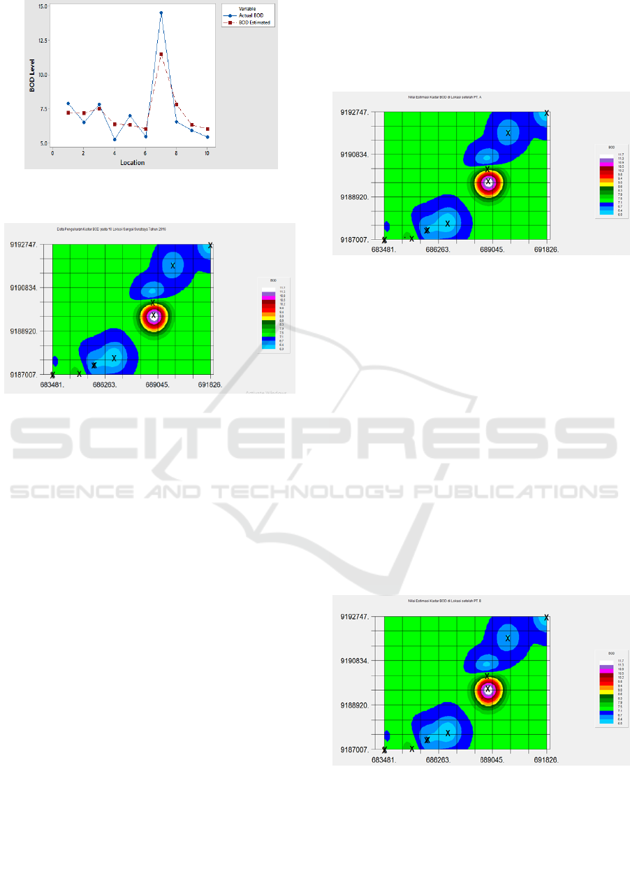
Figure 9: Plot Estimated Value and Actual Value of BOD
Level.
Figure 10: Estimated Spread of BOD Levels at Surabaya
River.
The BOD level in the lower reaches of the river is
low, this is due to the pollutant source from the
upstream of the river that leads to the downstream of
the river the smaller the effect.
The new location is estimated to be the location
points after the industries because according to the
ED information, the three industries are discharging
their waste into the channel that leads to the Surabaya
River. Selection of these location points is also due to
research by Suwari (2010), BOD level contributes a
large amount of industrial waste. Industrial waste
does not have high volume but its strongest
destructive power. The result of BOD level
estimation at the new location, namely location 11
with easting coordinate 684505 and northing
9187059 is presented in the form of a two-
dimensional contour map as figure 11.
The results show that BOD levels at location 11
around PT. An of 7.5 mg / l. This value was far
exceeding class II river water quality standard that
has been set at 3 mg / l, so that location 11 has been
contaminated status. There are several factors that
cause high levels of BOD in the location that is
because the river flow that still brings the influence of
waste from the previous location and also can be
expected because the location is close to PT. A which
is the industry with the dominant waste according to
Fardiaz (1992) that is hydrargyrum (Hg), cadmium
(Cd), chromium (Cr), lead (Pb), and copper (Cu).
This illustrates the industrial wastewater treatment
system of PT. A has not met the standard.
Figure 11: Estimated Spread of BOD Levels at Location 11.
Then the estimation of BOD levels in the new
location, namely location 12 with easting coordinate
and northing is presented in the
form of a two-dimensional contour map as figure 12.
The results show that BOD levels at location 12
around PT. An of 9.9 mg / l. This value is far
exceeding class II river water quality standard that
has been set at 3 mg / l, so that location 12 has been
contaminated status. Several factors cause high levels
of BOD in that location, which is due to river currents
that still carry the effect of waste from the previous
location including the waste of PT. A and may also
be suspected because the location of location 12 is
close to PT. B which is an industry with dominant
waste according to Fardiaz (1992), namely organic
matter, suspended solids (SS), dissolved solids (DS)
and Cd. This illustrates the industrial wastewater
treatment system at PT. B has not met the standard.
Figure 12: Estimated Spread of BOD Levels at Location 12.
ICMIs 2018 - International Conference on Mathematics and Islam
58

4 CONCLUSIONS
The result of modelling of sample BOD level using
cokriging method obtained by the best model based
on the smallest RSS value of 2838 is Gaussian model.
The value of
is very high of 91.5% and small MSE
value of 0.7057. This shows that the interpolation
results are accurate with the Gaussian model. The
estimation result of BOD level in Surabaya River
shows that BOD level leading downstream of the
river is lower. This is because the source of pollutants
from the upstream of the river that leads downstream
of the river is less have an effect. The results show
that BOD levels at new locationaroundPT. A, namely
location 11 of 7.5 mg / l. This value is far exceeding
class II river water quality standard that has been set
that is 3 mg / l so it can be said that the location has
been contaminated status.Several factors cause high
levels of BOD in the location that is because the river
flow that still brings the influence of waste from the
previous location and also can be expected because
the location is close to PT. A which is the industry
with the dominant waste that is hydrargyrum (Hg),
cadmium (Cd), chromium (Cr), lead (Pb), and copper
(Cu).Then the estimation of BOD levels in the new
locationaroundPT. A, namely location 12 of 9.9 mg /
l. This value far exceeding class II river water quality
standard that has been set that is 3 mg / l so it can be
said that the location has been contaminated status.
Several factors cause high levels of BOD in that
location, which is due to river currents that still carry
the effect of waste from the previous location
including the waste of PT. A and may also be
suspected because the location of location 12 is close
to PT. B which is an industry with dominant waste,
namely organic matter, suspended solids (SS),
dissolved solids (DS) and Cd.
REFERENCES
Ahmadi, S. H., and Sedghamiz, A., 2008. Application and
Evaluation of Kriging and Cokriging Methods on
Groundwater Depth Mapping. Journal Science, 138:
357-368, DOI 10.1007/s10661-007-9803-2.
Atima, W., 2014. BOD dan COD sebagai Parameter
Pencemaran Air dan Baku Mutu Air Limbah. Jurnal
Biology Science and Education, 3(2), ISSN 2252-858X.
Fardiaz, S., 1992. POLUSI AIR & UDARA, Penerbit
KANISIUS, Yogyakarta.
Haq, A. Z., 2017. Awas, Jangan Sembarangan Makan Ikan
Wader dan Mujaer dari Sungai Surabaya, SURYA,
March 8, 2017.
Isaaks, H. E. and Srivastava, R. M., 1989. Applied
Geostatistics. Oxford University Press, New York
Kelkar, M. and Perez, G., 2002. Applied Geostatistics for
Reservoir Characterization. Society of Petroleum
Engineers, USA.
Kis, I. M., 2016. Comparison of Ordinary and Universal
Kriging interpolation techniques on a depth variable (a
case of linear spatial trend), the case study of the
Sandrovac Field. Rudenko – Geolosko – Naftni Zbornik,
31(2), 41.
LeMay, N. E., 1995.Variogram Modeling and Estimation.
Thesis Master of Science Applied Mathematics,
University of Colorado, Denver.
Tchobanoglous, G., 1991. Wastewater Engineering
Treatment, Disposal, and Reuse, McGraw-Hill Book
Company, New Delhi.
Priyono, T. S. C., Yuliani, E. and Sayekti, R. W., 2013.
Studi Penentuan Mutu Air Sungai Surabaya untuk
Keperluan Bahan Baku Air Minum. Jurnal Teknik
Pengairan, 4(1): 53-60.
Razif, M. and Masduqi, A., 1996. Penelitian Korelasi COD
dan BOD Limbah Cair untuk Monitoring Pencemaran
Kali Surabaya. Majalah IPTEK, Mei.
Suwari, 2010. Model Pengendalian Pencemaran Air Pada
Wilayah Kali Surabaya. Dissertation, Institut Pertanian
Bogor.
Trisnawati, A. and Masduqi, A., 2013. Analisis Kualitas
dan Strategi Pengendalian Pencemaran Air Kali
Surabaya. Jurnal Purifikasi, 14(2): 90-98.
Biochemical Oxygen Demand Level Modeling in Surabaya River using Approach of Cokriging Method
59
