Energy Saving Potential Prediction and
Anomaly Detection in College Buildings
Nur Inayah, Madona Yunita Wijaya and Nina Fitriyati
Mathematics Program Study, Faculty of Sciences and Technology,
UIN Syarif Hidayatullah Jakarta, Jl. Ir. H. Juanda No. 95 Ciputat, Banten, Indonesia
Keywords: Artificial Neural Network, Energy Prediction, Hidden Markov Model, SARIMA, Stochastic Model
Abstract: Prediction of building electricity consumption has been studied in recent years. Several approaches have
been applied to get accurate and robust prediction of electricity usage. In this report, we highlight methods
to make buildings and college campus more efficient in using electricity through statistical modeling. We
focus on four main buildings in Syarif Hidayatullah State Islamic University Jakarta and collect each
building’s kWh energy consumption on a monthly basis. Two methods are utilized to the time series data,
SARIMA model and Artificial Neural Network (ANN) model. The ANN was found to have better model
performance than SARIMA with the smallest error prediction.
1 INTRODUCTION
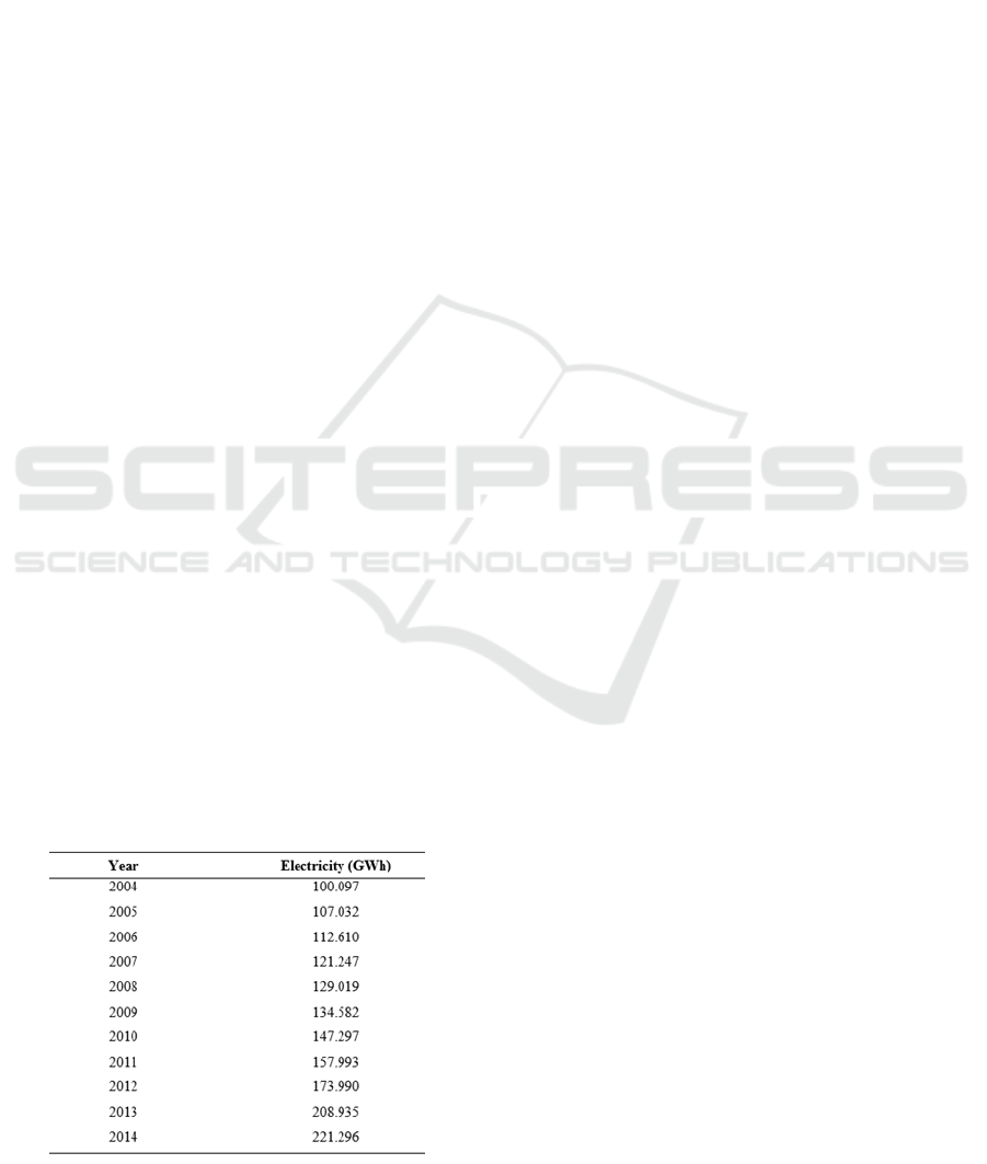
Electricity consumption throughout the world is
witnessing an increasing trend from year to year as
world population continues to grow. Electricity
consumption in Indonesia was reported to have
increased by an average 7% per year over period
2004 – 2014. This growth is led by increment of
household incomes as well as electrification ratio
(the percentage of households in Indonesia that are
connected to the nation’s electricity grid) and
therefore usage of electricity devices such as air
conditioners, refrigerators, etc. continue to rise.
Table 1: Electricity consumption from 2004 to 2014
(source: PLN statistics).
Another major area of concern is the production
of electricity and the environmental pollution that is
caused in the process of generating the electricity.
As we know, most of electricity that we use every
day for many purposes is generated using fossil
fuels. The basic power plants are thermal based and
depend on coal, diesel or other petroleum products
for converting water into high pressure stream which
is used to produce electricity through turbine-
generator mechanism. These fossil fuels are
predicted to become extinct in another 40-50 years.
Moreover, the amount of electricity use also
responsible for a significant proportion of total
carbon dioxide emissions. For these reasons,
management of energy consumption is a very
important issue to resolve the losses due to
consumption increment patterns and to lessen more
damage to environment. With regards to energy
management, our government have implemented a
number of policies including energy audit. Energy
audit is the process of evaluating energy utilization
and identifying chances for energy savings and also
recommending for improvement in energy efficiency
(PERMEN ESDM No. 14 2012).
Energy usage prediction in buildings has
received much consideration among researchers, as a
method to reduce consumption of energy, with
intention for energy savings and also to diminish
environmental impacts. These motivate us to study
Inayah, N., Wijaya, M. and Fitriyati, N.
Energy Saving Potential Prediction and Anomaly Detection in College Buildings.
DOI: 10.5220/0008516500150022
In Proceedings of the International Conference on Mathematics and Islam (ICMIs 2018), pages 15-22
ISBN: 978-989-758-407-7
Copyright
c
2020 by SCITEPRESS – Science and Technology Publications, Lda. All rights reserved
15

as well as to predict energy usage buildings
particularly at the UIN Syarif Hidayatullah
buildings. Activities inside buildings of UIN Jakarta
contribute a great proportion in using electricity,
especially to support teaching and learning activities.
In classrooms and administration buildings,
ventilation, lighting, and particularly cooling give
the biggest contribution for electricity consumption.
Therefore, these areas are the best targets for energy
savings. Another consideration is that many
universities, including UIN Syarif Hidayatullah,
have tight facility budgets, so finding lower cost
ways is a very important task to reduce energy bills.
We can also help campus to save energy expenses
by engaging faculty and students to involve in
energy efficiency. Therefore, through this research
study, we wish to model total electricity
consumption at the UIN Syarif Hidayatullah in order
to understand electricity consumption behaviour
over time and to accurately predict total
consumption in the future. Finally, we can use it as a
decision making to save energy and participate for
the world energy efficiency and particularly to
support our government policy for energy efficiency.
This report discusses the basics of electricity, its
measurement, worldwide trends with an emphasis on
methods that can be implemented to save electricity
especially in relation to the building and college
campuses.
2 PREDICTION MODEL
This section is devoted to describe the two
approaches used for energy prediction, i.e. SARIMA
and ANN. In the last part of this section, the method
for anomaly detection is discussed in details.
2.1 SARIMA Models
The Autoregressive Moving Average Models or also
known as ARMA model is a stationary process that
plays a key role in the modeling of time series data.
To motivate the model, for a series y
t
, the level of its
current observations can be modeled through the
level of its lagged distribution. This kind of model is
known as an autoregressive (AR) model. The AR(p)
model has order p and is expressed as follow:
In addition, we can also model the data at time t
where they are influenced by random innovation at
time t and the random innovation before time t. This
kind of model is known as a moving average (MA).
The MA(q) model has order q and is expressed as
follows:
.
If the two models are combined, we get a general
ARMA(p,q) with p AR terms and q MA terms:
.
Using ARMA processes, we can approximate
many real data sets in a more parsimonious way by a
mixed ARMA model that contains both AR and MA
process.
In real world setting, many time series data
shows non-stationary behavior. To model such
situation, Box and Jenkins (1976) formulated the
concepts of ARIMA. ARIMA is an acronym for
Autoregressive Integrated Moving Average Model.
This model has order p, d, and q and usually written
as ARIMA(p,d,q). We can express the model as
follows:
,
where
and d denotes the number of
differencing or integration order. We call this as an
ARIMA(p,d,q) model. If order of integration equals
to zero, then the original time series data is
stationary and ARIMA models come down to
ARMA models.
To account for seasonal behavior, Box and
Jenkins (1976) proposed SARIMA. In SARIMA
model, non-stationary can be eliminated from the
model by using the corresponding order of seasonal
differencing. The primary concept with seasonal
time series of period s is that the data with s intervals
apart are similar. The SARIMA model is generally
indicated as
, where
‘s’ denotes the seasonal period length, P is the
seasonal AR order, D is the seasonal integration
order, and Q is the seasonal MA order.
ICMIs 2018 - International Conference on Mathematics and Islam
16

2.2 Artifical Neural Networks
Artificial neural networks (ANNs) have received
much interest in the past few years. It is a relatively
new approach that can handle complex situation and
offer flexibility for prediction and classification as
compared to traditional statistical approach such as
regression (Cheng and Titterington, 1994). ANNs
provide alternative solution to model non-linear data
and have been used among researchers to solve
energy prediction problem (Bishop, 2007).
ANN method comprises three important
features. The first feature is neurons or nodes. It is
the elementary processing elements in ANN. The
basic processing elements, or neurons, are arranged
in layers. The layers between the input and the
output layers are called hidden layers. The second
feature is the network architecture. It explains the
connections between neurons. Finally the last feature
is the training algorithm. The network parameter
values are searched by this training algorithm to
work a specific task for classification (Allende et al.,
2002). A neural network class can be defined by the
following expression:
,
where
is a non-linear function of , is the
number of hidden neurons is the vector of
parameter, and is the number of free parameters
that is determined by
, i.e.
.
A trained ANN method needs the performance
error to convergence to a unique minimum (local).
For any particular topology
, where a trained
network has to convergence, we introduce the
requirement and a restricted search is performed in
the function space. The general algorithms of ANN
are summarized in the following:
1. The parameters in the model is estimated by
minimizing the empirical loss
iteratively.
2. The error Hessian
is computed to carry on
convergence test.
3. Matrix
is examined to check if it has negative
eigen values. This is used to perform
convergence and uniqueness test.
4. The prediction risk
is estimated
which adjust the empirical loss for complexity.
5. The model is selected by using the principle of
minimum prediction risk. This expresses the
trade-off between the generalization ability of
the network and its complexity.
2.3 Statistical Measure
A good learner (model) is the one which has good
prediction accuracy. In other words, it has the
smallest prediction error. In this study, several
statistical measures are used such as MAPE, MAD,
and RMSE.
The mean absolute percentage error (MAPE) is a
measure of prediction accuracy of a forecasting
method and can be expressed as:
where is the number of sample data,
is the
actual data on time i,
is the predicted data on
time i.
The mean absolute deviation (MAD) is defined
as an error statistic that average the distance between
each pair of actual and fitted data points. The
formula for calculating MAD is given as:
.
The root mean squared error (RMSE) is an
absolute error measures the squares the deviations to
keep the positive and negative deviations from
cancelling one another out. This measure also tends
to exaggerate large errors, which can help when
comparing methods. The formula to calculate RMSE
is given as:
.
2.4 Anomaly Detection
The selected model with the highest prediction
accuracy according to MAPE criteria will be used to
detect anomaly. The basic idea is to use the model to
predict the electricity consumption on time t. If the
difference between the observed and the predicted
value is greater than a certain threshold we classify it
as an anomaly (Halldor et al, 2014). The error is
defined as follows:
.
A sample will be classified an anomaly if the
error is above a certain threshold. This threshold
value can be determined through an experiment.
Intuitively, a value is considered an outlier if its
Energy Saving Potential Prediction and Anomaly Detection in College Buildings
17
error is higher than the other errors. Three-sigma-
rule will be considered in this research as the
threshold. If the error of a sample data is greater than
three times the standard deviation then it will be
classified as an anomaly.
3 EXPERIMENT AND RESULTS
3.1 Exploratory Data Analysis
Data for electricity consumption at the UIN Syarif
Hidayatullah buildings were collected from the 4
main buildings:
1. Rectorate building.
2. Campus 1 (main campus that consists of
Tarbiya and Teaching Sciences Faculty,
Shari’a and Law Faculty, Dirasat Islamiyah
Faculty, Da’wa and Communications Faculty,
Adab and Humanities Faculty, Usul al-Din and
Philosophy Faculty, Economics and Business
Faculty, and Science and Technology Faculty)
3. Campus 2 (located on Kertamukti Street that
consists of Faculty of Psychology and Faculty
of Social and Political Science)
4. Campus 3 (located on Kertamukti street that
consists of Faculty of Medical and Health
Science)
The data were measured in kWh (kilowatt hours)
and were collected in 56 months from January 2013
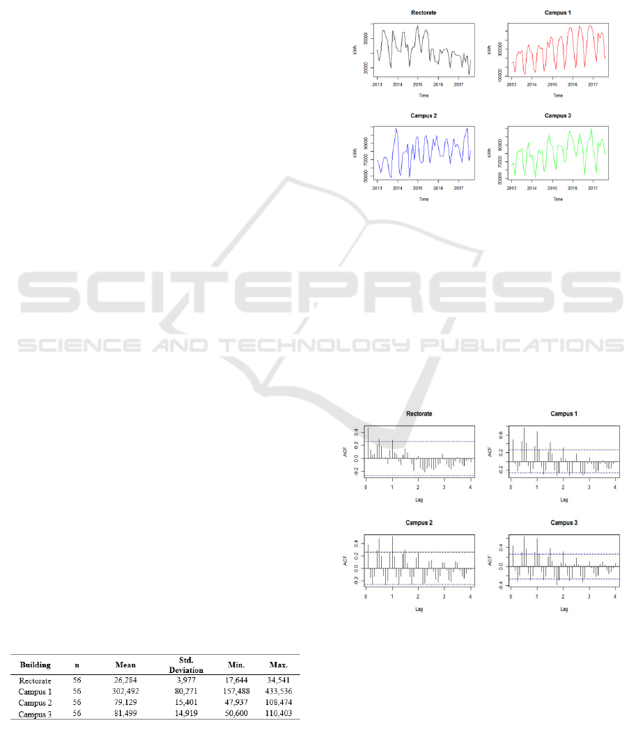
to August 2017. Figure 1 displays the energy
consumption profiles of electricity consumption in
the four buildings over the months. It shows that
Campus 2 and Campus 3 behave relatively similar
from month to month. The plots also indicate
fluctuations as well as seasonal pattern in the
monthly energy consumption. One can see that there
is greater energy consumed during teaching periods
due to increased use of the lighting and air
conditioning in classes. The least energy consumed
happened during semester break when normal
classes are not conducted. It can also be observed
that energy consumptions were slightly increased
over the years for Campus 1, 2, and 3 but showed a
decreasing trend for Rectorate building starting from
middle of year 2015.
Table 2: General characteristics of data sets.
Table 2 summarizes their respective descriptive
statistics. As can be expected, Campus 1 used the
largest energy by 302,494 kWh on average since
Campus 1 is the main building that consists of many
faculties. The second and the third largest were
Campus 3 (81,499 kWh) and Campus 2 (79,129
kWh), respectively. Rectorate building consumed
the least by 26,284 kWh.
Figure 1: Electricity consumption profile over the months.
3.2 SARIMA Models
Visual examination of Figure 1 shows that the
process is non-stationary with both trend and
seasonality components. This is also confirmed from
the ACF plots (Figure 2) that clearly show the
existence of strong seasonal dependency with high
coefficients in 12, 24, 36, and so on which fade
slowly with the lag.
Figure 2: Plot of ACF of the time series data.
Table 3 also confirms that the data is non-
stationary by using three different methods (ADF,
KPSS and PP tests). The ADF test is not significant,
meaning the null hypothesis of unit root cannot be
ICMIs 2018 - International Conference on Mathematics and Islam
18
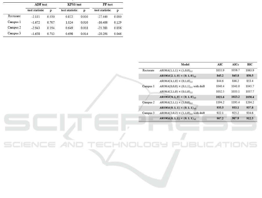
rejected. The results of KPSS tests are significant
meaning the null hypothesis of stationary process is
rejected. Therefore, we need to take first difference
to the time series data. The general upward trend has
disappeared after we take first difference to the data
but the strong seasonality is still present.
Table 3: ADF, KPSS, and PP tests for the time series data.
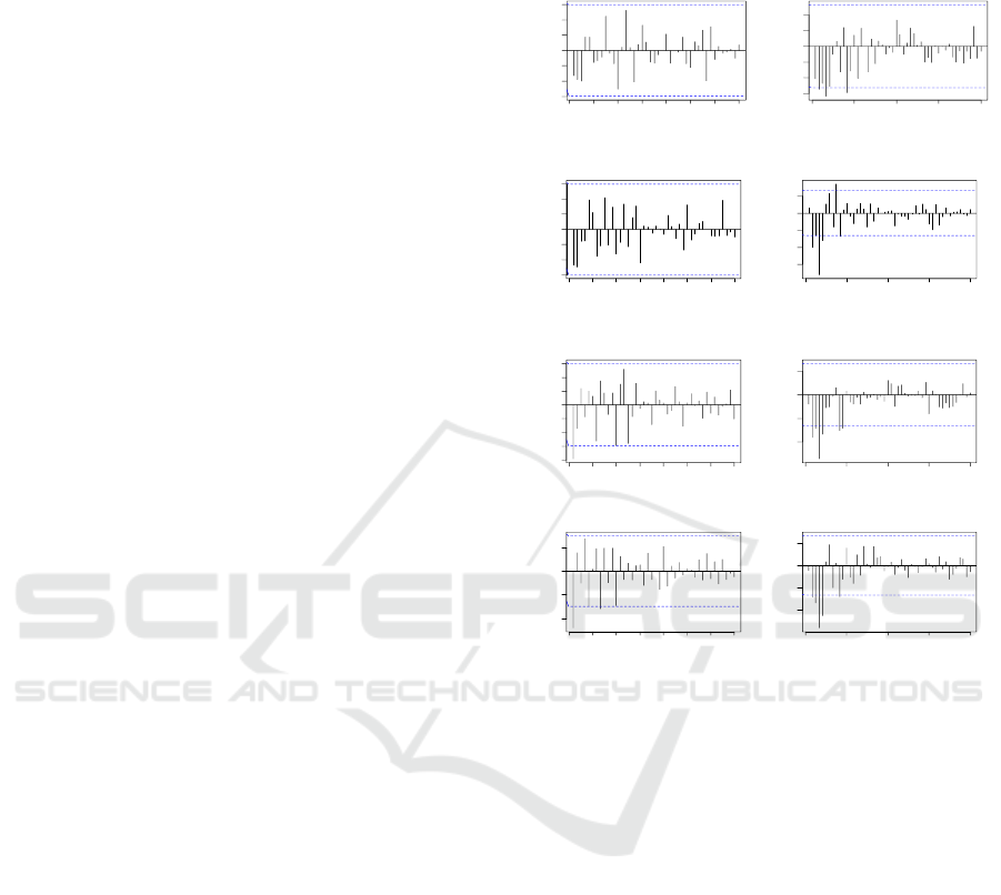
Observing both ACF and PACF plots of the
series after taking first and seasonal difference (see
Appendix), we come up with several potential
models for each building as summarized in Table 4.
For electricity consumption pattern in Rectorate
building, the PACF shows a clear spike at lag 2 or 4.
A non-seasonal AR(2) or AR(4) may be useful part
of the model. In the ACF, there appears no
significant lag. Thus, the proposed model for the
series of electricity consumption in Rectorate
building is
or
.
For electricity consumption pattern in Campus 1
building, the PACF also shows a clear spike at lag 2
or 4. A non-seasonal AR(2) or AR(4) may be useful
part of the model. Thus, the proposed model for the
series of electricity consumption in Campus 1
building is
or
.
For electricity consumption pattern in Campus 2
building, the ACF shows a clear spike at lag 1. A
non-seasonal MA(1) may be useful part of the
model. In the PACF, there’s a cluster of (negative)
spikes around lag 12 and then not much else. This
might indicate the need for a seasonal MA(1)
component. Thus, the proposed model for the series
of electricity consumption in Campus 2 building is
.
For electricity consumption pattern in Campus 3
building, the ACF shows a clear spike at lag 1. A
non-seasonal MA(1) may be useful part of the
model. In the PACF, there’s a cluster of (negative)
spikes around lag 12 and then not much else. This
might indicate the need for a seasonal MA(1)
component. Thus, the proposed model for the series
of electricity consumption in Campus 2 building is
.
Automatic procedure to select the order of
seasonal and non-seasonal component was also
performed with R by using auto.arima function. The
comparisons of the proposed models are shown in
Table 4.4. Based on AIC and BIC values, the best
fitted model for electricity consumption pattern in
Rectorate building is
.
The best fitted model for electricity consumption
pattern in Campus 1 building is
with drift. The best fitted model for
electricity consumption pattern in Campus 2
building is
. The best
fitted model for electricity consumption pattern in
Campus 3 building is
.
Table 4: AIC and BIC comparison for the proposed
models.
Based on AIC and BIC values, the best fitted
model for electricity consumption pattern in
Rectorate building is
.
The best fitted model for electricity consumption
pattern in Campus 1 building is
with drift. The best fitted model for
electricity consumption pattern in Campus 2
building is
. The best
fitted model for electricity consumption pattern in
Campus 3 building is
.
Using the Maximum Likelihood estimator, the
model parameters are estimated. Table 5 summarizes
the estimated coefficient and standard error of the
best fitted seasonal ARIMA models.
Diagnosis analyses are also performed to the four
models to evaluate the model assumption such as no
correlation in the residual series. Assumption of no
correlation in residuals is investigated by performing
Ljung-Box test (Table 6). The result of Ljung-Box
for the residual series from the model fitted to the
Rectorate data are not significant since the test fails
reject the null hypothesis of no autocorrelation in the
residual series (p = 0.422). The result of Ljung-Box
for the residual series from the model fitted to the
Campus 1 data are not significant since the test fails
reject the null hypothesis of no autocorrelation in the
Energy Saving Potential Prediction and Anomaly Detection in College Buildings
19
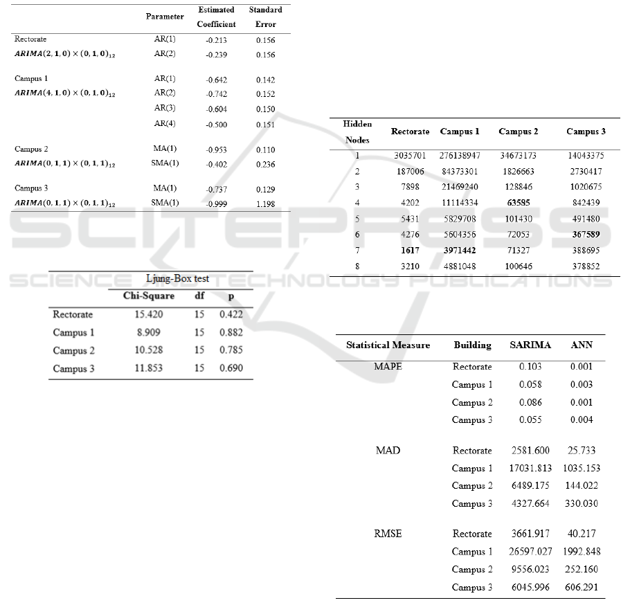
residual series (p = 0.882). The result of Ljung-Box
for the residual series from the model fitted to the
Campus 2 data are not significant since the test fails
reject the null hypothesis of no autocorrelation in the
residual series (p = 0.785). The result of Ljung-Box
for the residual series from the model fitted to the
Campus 3 data are not significant since the test fails
reject the null hypothesis of no autocorrelation in the
residual series (p = 0.690). Thus, we can conclude
that there is no autocorrelation in the residual series.
Table 5: The estimated parameters of seasonal models.
Table 6: The estimated parameters of seasonal models.
3.3 ANN Models
The ANN models are also fitted to the time series
data using feed-forward with multilayer perceptrons
(MLP). Mean square error (MSE) is used as a
criteria for model selection according to the number
of hidden nodes. MSE measures how good the fitted
model by computing how many errors it makes. The
lower the MSE score, the better the model. Table 7
reveals that ANN model 7 hidden nodes is
appropriate to model kWh consumption in both
Rectorate and Campus 1 buildings. ANN model with
4 hidden nodes is appropriate to model kWh
consumption in Campus 2 building. ANN model
with 6 hidden nodes is appropriate to model kWh
consumption in Campus 3 building.
3.4 Model Comparison
Table 8 summarizes the comparison of
forecasting precision between the two methods
according to MAPE, MAD, and RMSE criteria.
Empirical results on the four data set by utilizing
two different approaches clearly show the efficiency
of the ANN model since the values of MAPE, MAD,
and RMSE are the lowest. Figure 3 displays the
comparison between actual data and fitted values
based on SARIMA and ANN. The plots also
confirm that ANN is the best model since it can
approximately predict the true values, the ANN lines
are almost overlap with the actual lines.
Table 7: Comparison of MSE scores for the different
hidden nodes in ANN model.
Table 8: Comparison of MAPE, MAD, and RMSE.
ICMIs 2018 - International Conference on Mathematics and Islam
20
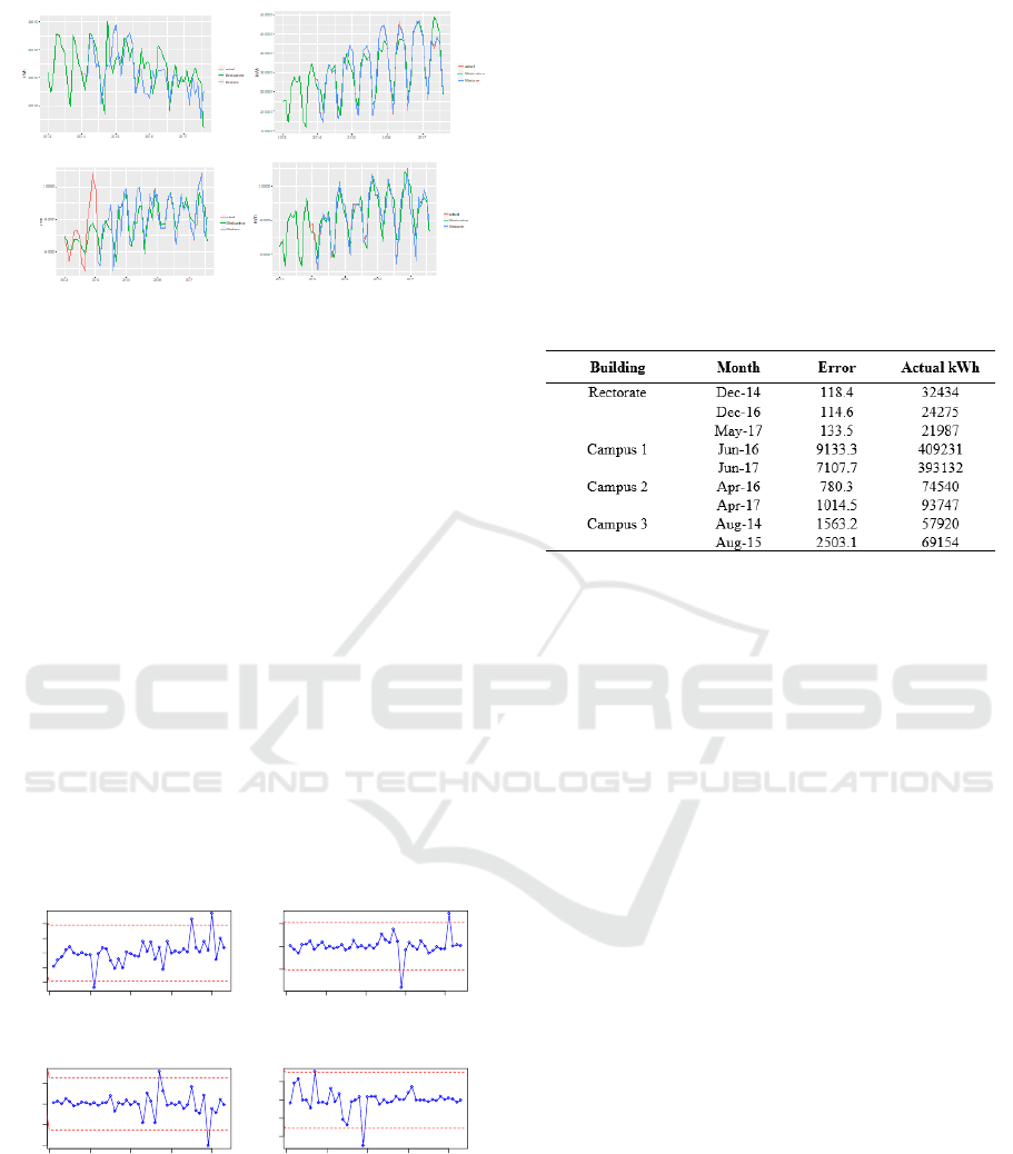
Figure 3: Plot of actual vs. predicted value based on
SARIMA and ANN model for Rectorate (top left),
Campus 1 (top right), Campus 2 (bottom left), and
Campus 3 (bottom right).
3.5 Anomaly Detection
Figure 4 shows the monthly analysis for the anomaly
detection set. The threshold (red dashed line) is
calculated from the standard deviation of the error,
where error is calculated as the absolute value of the
difference between the actual and the predicted kWh
consumption. If the error is greater than 3σ or less
than -3σ, we detect the series as outlier or anomaly
data. From the Rectorate dataset, there are 3
anomaly data. From Campus 1 dataset, there are 2
anomaly data. From Campus 2 and 3 dataset, there
are 2 anomaly data for each. In total, there are 9
anomalies detected from all buildings. These
anomalies are further listed in Table 9 because their
calculated errors are greater than three-sigma-rule.
Figure 4: Plot of anomaly detection.
In June 2017, the actual consumption in Campus
1 building was 393,132 kWh and the model predicts
7107.7 kWh lower than what was recorded. These
kind of anomalies found in Campus 1 are peak
anomalies and were found during semester break
where electricity consumption should be generally
lower than semester dataset (classes) since there is
no activities inside campuses especially for teaching
and learning activities. Logical explanation for this
peculiar behaviour could be due to waste of energy
such as usage of electricity components (like air
conditioner, etc.) when there are no activities inside
the building. There are however many significant
peak anomalies in the data that cannot be explained
due to very limit source of information from
secondary data and need further investigation.
Table 9: The listed anomalies from the four buildings.
4 CONCLUSIONS
From statistical point of view and by considering
electricity consumption data at the UIN Syarif
Hidayatullah building, two different approaches
were conducted to analyze the behavior of energy
usage over time in the four main campuses building.
According to the electricity consumption trend
found in the data, the behavior of electricity
consumption in the four buildings can be categorized
into two states, i.e. high demand during class
semester and low demand during semester break.
This is a very logical explanation because during
class semester, activities inside campuses will
increase so electricity demand will also increase.
Higher consumptions will be for lighting and
cooling to support teaching and learning activities.
The demand will be low when there is no class
during semester break; therefore electricity
consumption will be relatively low.
In terms of energy prediction, the results indicate
that artificial neural network outperforms the other
methods, with the smallest MAPE values. This
shows that ANN can best approximately the
electricity usage in the future. From the forecast
plot, we can see that electricity consumption will
increase in the near future. From the anomaly
detection section, we could only point several peak
anomalies during semester break. This, of course,
0 10 20 30 40
-100
0 50
Rectorate
time
E
0 10 20 30 40
-5000
0 5000
Campus 1
time
E
0 10 20 30 40
-1000
0 500
Campus 2
time
E
0 10 20 30 40
-2000
0 1000
Campus 3
time
E
Energy Saving Potential Prediction and Anomaly Detection in College Buildings
21
need further investigation because it could lead to
energy efficiency.
REFERENCES
Allende, H., Moraga, C., and Salas, R., 2002. Artificial
neural networks in time series forecasting: a
comparative analysis. Kybernetika, 88, pp. 685–707.
Baum, L. E. and Petrie, T., 1996. Statistical inference for
probabilistic functions of finite state markov chains.
Annals of Mathematical Statistics, 37, pp. 1559–1563.
Bishop, C. M., 2007. Pattern Recognition and Machine
Learning (Information Science and Statistics), 1
st
ed.
Springer.
Box, G. E. P. and Jenkins, G. M., 1976. Time Series
Analysis, Forecasting and Control. San Francisco:
Holden–Day.
Cheng, B. and Titterington, D.M., 1994. Neural networks:
review from a statistical perspective. Statistical
Science (1), pp. 2–54.
Halldor, J., Florian, S., Sebastian, M., and Daniel, A.K.,
2014. Anomaly detection for visual analytics of power
consumption data. Computers & Graphics, 38, pp. 27–
37.
Kalogirou, S. A., 2016. Artificial neural networks in
energy applications in buildings. International Journal
of Low–Carbon Technologies, vol. 1, no. 3, pp. 201–
216.
Khosravani, H.R., Castilla, M.D.M., Berenguel, M.,
Ruano, and A.E., Ferreira, P.M., 2016. A Comparison
of Energy Consumption Prediction Models Based on
Neural Networks of a Bioclimatic Building. Energies,
9, p. 57.
Suganthi, L. and Samuel, A. A., 2012. Energy models for
demand forecasting—A review. Renew. Sustain.
Energy Rev., 16, pp. 1223–1240.
The Oxford Institute of Energy Studies, 2017. Indonesia’s
Electricity Demand and the Coal Sector: Retrieved
from: https://www.oxfordenergy.org/ wpcms/wp-
content/uploads/2017/03/Indonesias-Electricity-
Demand-and-the-Coal-Sector-Export-or-meet-
domestic-demand-CL-5.pdf, on Oct 2017.
Wong, S., Wan, K. K., and Lam, T. N., 2010. Artificial
neural networks for energy analysis of office buildings
with daylighting. Applied Energy, vol. 87, no. 2, pp.
551–557.
Zaid, M. and Bodger, P., 2014. Forecasting Electricity
Consumption: A Comparison of Models for New
Zealand.
Zia, T, Bruckner, D., and Zaidi, A., 2011. A hidden
markov model based procedure for identifying
household electric loads. IECON 2011 - 37th Annual
Conference on IEEE Industrial Electronics Society,
pp. 3218–3223.
APPENDIX
Figure: ACF and PACF of first and seasonal difference of
kWh consumption in the four buildings.
0.0 0.5 1.0 1.5 2.0 2.5 3.0 3.5
-0.3
-0.1
0.0
0.1
0.2
0.3
ACF of first and seasonal diff. - Rectorate
Lag
ACF
0 1 2 3 4
-0.3
-0.2
-0.1
0.0
0.1
0.2
Lag
Partial ACF
PACF of first and seasonal diff. - Rectorate
0.0 0.5 1.0 1.5 2.0 2.5 3.0 3.5
-0.3
-0.1
0.0
0.1
0.2
0.3
ACF of first and seasonal diff. - Campus 1
Lag
ACF
0 1 2 3 4
-0.6
-0.4
-0.2
0.0
0.2
Lag
Partial ACF
PACF of first and seasonal diff. - Campus 1
0.0 0.5 1.0 1.5 2.0 2.5 3.0 3.5
-0.4
-0.2
0.0
0.2
ACF of first and seasonal diff. - Campus 2
Lag
ACF
0 1 2 3 4
-0.4
-0.2
0.0
0.2
Lag
Partial ACF
PACF of first and seasonal diff. - Campus 2
0.0 0.5 1.0 1.5 2.0 2.5 3.0 3.5
-0.4
-0.2
0.0
0.2
ACF of first and seasonal diff. - Campus 3
Lag
ACF
0 1 2 3 4
-0.4
-0.2
0.0
0.2
Lag
Partial ACF
PACF of first and seasonal diff. - Campus 3
ICMIs 2018 - International Conference on Mathematics and Islam
22
