A Comparison of Tidal Zoning Model for the Depth Reduction

Danar Guruh Pratomo

, Eko Yuli Handoko

and Duty Kendartiwastra

Geomatics Engineering Department, Faculty of Civil Engineering, Environment, and Geo-Engineering, Institut Teknologi

Sepuluh Nopember, Surabaya, Indonesia

Keywords: Tidal Zoning, Tidal Constituent, Residual Interpolation

Abstract: Bathymetric information is essential for navigational purpose. The depth in navigational charts has to be

referred to a vertical datum with the intention of ships can navigate safely. Tide plays important rule in a depth

reduction in order to provide bathymetric information. Tidal characteristics are unique for any different places.

The tidal phase and amplitude propagation may cause difficulties in predicting water levels. The research

utilized Tidal Constituent and Residual Interpolation methods to estimate the tide propagation and to achieve

a smooth tidal zoning. Tidal constituents at each of observation point are calculated using the least squares

method and interpolated based on Laplace formula. The tidal zoning model that has been developed then was

compared to the Finite Element Solution 2014 Global Tide Model. The results show that the correlation

coefficient between those models is 0.78. Based on the research, the tidal zoning model can be used to improve

the global tide model.

1 INTRODUCTION

Seafloor information is important for supporting

marine activities (safety of navigation, demersal

fishing, offshore oil exploration and drilling, cable

and pipeline laying maintenance, and underwater

warfare). A depth measurement is the main activity to

determine the topography of the seabed. The

measured depth must be corrected by the tides so that

it refers to a chart datum. Corrected depths are the

basic information to generate a nautical chart. The

chart can also be utilized for a shipping safety and

construction of docks purposes. Due to the

importance of a chart datum in reducing depth, the

determination of the vertical datum must be

conducted accurately and precisely (Hellequin, et.al,

2003). The accuracy of a chart datum in a certain area

depends on the tide observation process and the

determination of tidal characteristics. The range

between tidal stations or between tidal station and

survey area may also affects the accuracy as it creates

a tide zonation. The determination of the tide zonation

can improve the accuracy of the tide correction for the

depth reductions.

The study discussed the simulation of a tidal

zoning using the TCARI (Tidal Constituent and

Residual Interpolation) approach. TCARI uses an

interpolation method from tide data at several tide

stations. The method applies Laplace equation to

simulate the tide on a weighted grid area model

(Cisternelli and Gill, 2005). Each point on grid has a

unique tide phase and amplitude which can be used to

predict the water level at a certain position and time.

The advantage of this approach is that the

discontinuities of the tide observation which occur in

the transition zone can be eliminated. The method can

separate the calculation of water level due to tidal and

non-tidal effects (weather and river discharge) and

can also display model uncertainty due to tidal datum,

astronomic, and water level uncertainty errors

(Cisternelli, et.al, 20017).

The research also examined the results of the tide

model from TCARI and the Finite Element Solution

2014 global tide model (FES2014). FES2014

represents tidal cycles across the globe. This model is

derived from several altimetry satellite missions

(Cancet, et.al, 2017). Based on the comparison

between these models, it is expected that tide model

from TCARI can improve the accuracy and the

resolution of the global tide model FES2014

especially on the coastal area.

Pratomo, D., Handoko, E. and Kendartiwastra, D.

A Comparison of Tidal Zoning Model for the Depth Reduction.

DOI: 10.5220/0008373900500054

In Proceedings of the 6th International Seminar on Ocean and Coastal Engineering, Environmental and Natural Disaster Management (ISOCEEN 2018), pages 50-54

ISBN: 978-989-758-455-8

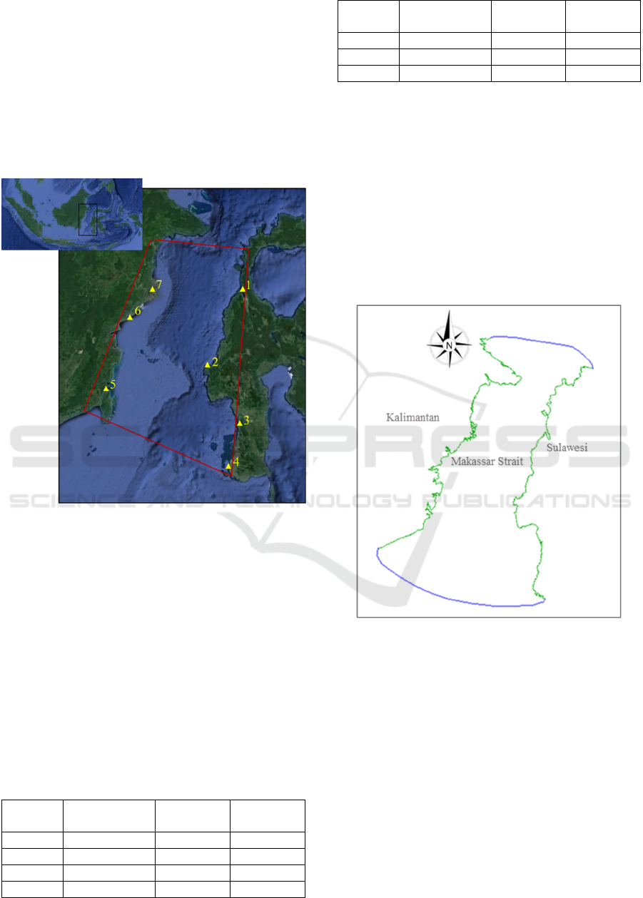
2 METHODS

The research is located in Makassar Strait, the strait

between Kalimantan and Sulawesi which is

connected to Pacific Ocean in the north and adjacent

with Java Sea in the southern part. The geographical

location of the research area stretches from

115°25'03.7"E to 120°00'34.8"E of the longitude and

from 05°30'04.8"S to 00°57'52.36"N of the latitude

(red line in Fig. 1).

Figure 1: The research area located in Makassar

Strait

The research used 7 tide stations in the proximity

of the area of interest (yellow triangles in Fig. 1). The

tide observations data from these stations are

provided by Indonesia Geospatial Information

Agency (2017). The data is then processed based on

10 minutes to obtain tide constituents at each tide

stations. The geographical coordinates of the tide

stations can be seen in Table 1.

The tide constituents from the tide stations are

interpolated using TCARI method. The Pydro

(Python and Hydrography) software was utilized to

generate the tidal zoning in TCARI method.

Table 1: Tide Station Coordinate

Number Station Name

Easting

(dec deg)

Northing

(dec deg)

1 Pantoloan 119.857E -0.712S

2 Mamuju 118.893E -2.667S

3 Pare-pare 119.620E -4.014S

4 Makassar 119.417E -5.112S

Number Station Name

Easting

(dec deg)

Northing

(dec deg)

5 Kota Baru 116.146E -3.291S

6 Balikpapan 116.806E -1.272S

7 Mahakam 117.399E -0.553S

The boundary for the model is derived from the

medium resolution of GSHHG. The GSHHG is a

high-resolution geography data set, amalgamated

from World Vector Shorelines (WVS) and CIA

World Data Bank II (WDBII) (Wessel and Smith,

1996). The data contains coastline and islands in shp

format. The model boundary for the model is a closed

polygon. The open ocean boundary for the model is

delineated from the area which is adjacent with

Pacific Ocean and Java Sea. In Fig. 2 shows the

coastal boundary is represented by green line and the

open ocean boundary is represented in blue line.

Figure 2: The boundary of the model

Tidal constituents at each tide station are arranged

in a .txt file in a format that can be read in Pydro. The

file also includes additional information such as the

results of vertical datum calculations (MHHW,

MHW, MLW, MLLW, and MSL). In this case MSL

(Mean Sea Level) was used as a vertical reference for

each tide stations. Note that amplitude and phase

formats follow the format from NOAA and for

constituents with 0 value will not be modeled. This

research used 11 tidal constituents; K1, O1, P1, M4,

MS4, MF, MM, M2, S2, K2, and N2.

There are several tide stations located not exactly

at the shoreline, due to the shoreline resolution. Thus,

the position of the station is shifted so that it intersects

A Comparison of Tidal Zoning Model for the Depth Reduction

to the shoreline. This used an assumption that the

shifting positions have the same tide regime with the

tide actual stations.

The model used TIN (Triangular Irregular

Network) with 9900 nodes and approximately

255268.763 square kilometers of model domain. The

distribution of nodes is organized so that areas close

to the shoreline and islands’ boundaries have denser

distribution than other areas. The nodes distribution

for the model can be seen in Fig. 3. The nodes

distribution considers geometry of the beach, bay, and

headland which affect local effects such as wind and

currents which indirectly influence the hydrodynamic

characteristics in the research area.

Figure 3: The distribution of nodes used in the

model

The tidal amplitude and phase from each tidal

station are interpolated and iterated using Laplace

formula. The calculation process was performed for

each node. To speed up the iteration and effectiveness

of storage space (memory), the formula is simplified

as follows (Cisternelli, et.al, 2007):

(1)















= 0 (2)









,



,



 (3)

Where m is the index of the tidal stations, G is the

value of the amplitude and phase at a node and x, y is

the position of the node in cartesian coordinates

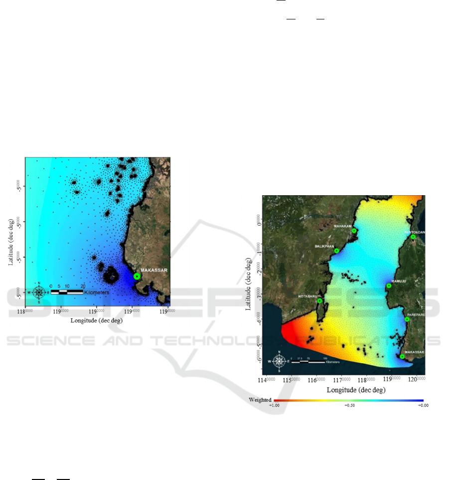
system which will be calculated its magnitude. A

weighted parameter was applied to improve the

equation. The weighted parameter was generated

based on the boundary configuration. The following

formula shows the weighted parameter applied in

Laplace formula:





0 (4)









(5)

01

Formula 4 was applied at points located on the

coastline where the interpolated value is known.

Formula 5 was applied at points where interpolation

values want to be determined. is the direction of a

node with respect to a shoreline. α is a constant which

affects the contour. The weighted parameter ranges

from 0 to 1. The farther from the tide station, the

weighted value will be close to 1. This means the

predictive data is more accurate when the radius of

the place to the tide observation point gets closer.

Thus, this range can be a representation of the

uncertainty level of the tide model. Fig. 4 shows the

weighted distribution of the model.

Figure 4: Weighted distribution of the model

The step after a computation using Laplace

formula is extracting the co-amplitude and co-phase

of the tide using TCARI. The co-amplitude and co

phase of every tidal constituents are computed using

interpolation method. Fig. 5 is one of the example of

the co-amplitude and co-phase from K1 constituent.

This co-tidal chart of K1 constituent is created using

TCARI method. The co-amplitude is represented with

colors gradation and the co-phase is represented by

white lines. Other tide constituents are extracted

using the same technique used to develop the K1 co-

tidal chart.





,



,,



1





ISOCEEN 2018 - 6th International Seminar on Ocean and Coastal Engineering, Environmental and Natural Disaster Management

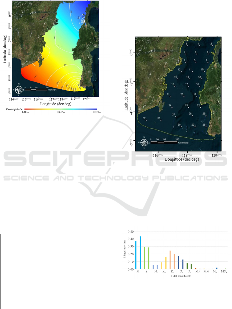
Figure 5: Co-amplitude and co-phase of K1

3 RESULT AND DISCUSSION

The research compared the tide model from TCARI

to the FES2014 model. The comparation is performed

to analyze the co-tidal chart pattern of each model.

This process aims to test the quality of the TCARI

tide model. FES2014 is developed from tide

observation data collected using satellite altimetry

whereas TCARI is generated by interpolating in-situ

data. Both models should show the same tide pattern

in the research area. However, these methods have

weaknesses and strengths which can be seen in Table

Table 2. Comparation between FES2014 and TCARI

Parameter FES2014 TCARI

Observation

Time

Interval

Depend on cycle

period of satellite

altimetry mission

Up to 1 hour

Quality base

characteristic

area

Good in off-shore,

not really good in

near-shore.

Good in near-

shore and not

really good in

off-shore.

Observation

Continuity

Consistent (for

along years)

Inconsistent

(depends on tide

gauge

accuration)

Scale Global Local to Global

The difference in Table 2 causes inconsistent

variations in TCARI and FES2014 tide constituent

values, depending on the position of the points

compared. Correlation values were obtained from 32

Independent Check Points that had been spread

evenly in the study area as in Fig. 6.

Figure 6: Independent Check Points

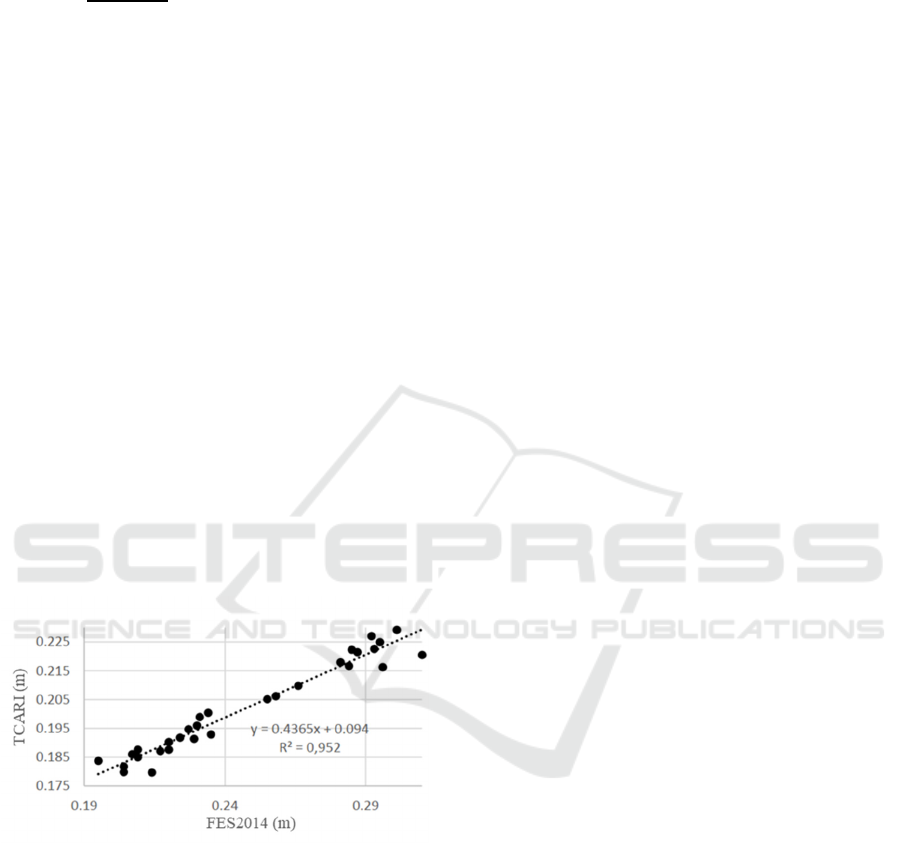
Figure 7 shows the average between the FES2014

and TCARI amplitude values for each tidal

constituent at 32 ICP points. The correlation

coefficient shows a strong relationship to the diurnal

and semidiurnal tidal constituents. Whereas for the

long period tidal constituents between TCARI and

FES2014 have magnitude close to 0 (Fig. 7).

Figure 7: Average of Amplitude Value in

Independent Check Points

The small values of the MS4, M4, MF and MM

constituents are influenced by Rayleigh criteria. The

Rayleigh criteria is if there are two components A and

component B can only be separated if the length of

the data is more than a certain period called the

A Comparison of Tidal Zoning Model for the Depth Reduction

synodic period. The synodic period can be formulated

by the following formula (Hess, 2004):

(7)

PS= Synodic Period (hours)

= Angular Velocity of A Component (ͦ /hour)

= Angular Velocity of B Component (ͦ /hour)

Based on the formula 7, the observed period

values for distinguishing spectral MS4 and M4 are

4.310 months and for distinguishing MF and MM

spectral, a minimum observation time of 27.076 days

is required. Thus, because the length of observation

used varies at each station, which is only about 3 to 7

months, it is considered less ideal for extracting the

M4 and MS4. However, this is ideal for extracting

MM and MF. The small MM and MF magnitudes are

possibly caused by other factors, for example the

influence of the position of the Makassar Strait which

is located at the equator. Considering that MM and

MF are long-term conditions that are influenced by

the declination of the moon, this made MM and MF

are minimum at near equator. Based on 11 tidal

constituents that have been modelled, the K1 has a

strongest correlation between TCARI and FES2014.

Fig 8 shows the coefficient correlation between the

models. The magnitude of their correlation is 0.976.

Figure 9: The coefficient correlation between

TCARI and FES2014 for K1 constituent

4 CONCLUSION

The tidal zoning model generated using the TCARI

method was compared with the global tide model

FES2014 to test the accuracy and precision of the

model. Based on the correlation test that has been

carried out on both models, the tide constituents of

S2, N2, K2, K1, O1, P1, and M2, have correlation

coefficient of 0.78. The best correlation is shown by

the pattern of K1 values with a correlation coefficient

of 0.95. The TCARI method can display smoother

tide models than the global tide model FES2014.

Tidal zoning model developed using TCARI might be

used to improve the resolution of global tide models

for the future purposes.

REFERENCES

K. Hess, 2004. NOAA technical report NOS CS. V 4.

L. Hellequin, J.M. Boucher, X. Lurton, 2003. IEEE J.

Oceanic Eng. E 28, 1.

M. Cisternelli, S. Gill, 2005. U.S. Hydrographic

Conference.

M. Cisternelli, C. Martin, B. Gallagher, R. Brennan,

2007. U.S. Hydrographic Conference.

M. Cancet, F. Lyard, D. Griffin, L. Carrère, N. Picot,

2017. 10th Coastal altimetry workshop, Italy.

Indonesia Geospatial Information Agency, 2017.

http://tides.big.go.id.

P. Wessel, W. H. F. Smith, 1996. J. Geophys. Res., B

4, 101, pp. 8741-8743.

 

360









ISOCEEN 2018 - 6th International Seminar on Ocean and Coastal Engineering, Environmental and Natural Disaster Management