Nonlinear Subband Spline Adaptive Filter

Chang Liu, Xueliang Liu

, Zhi Zhang and Xiao Tang

School of Electronic Engineering, Dongguan University of Technology, No.1 DaXueRoad, Dongguan, China

chaneaaa@163.com, liuxueliang83@163.com ,{zhangz, tangx}@dgut.edu.cn

Keywords: Subband adaptive filter, Nonlinear spline adaptive filter, adaptive filter algorithm, system identification.

Abstract: It has been reported that a novel class of nonlinear spline adaptive filter (SAF) obtains some advantages in

modeling the nonlinear systems. In this paper, a nonlinear subband structure based on the spline adaptive

filters, called subband spline adaptive filter (SSAF) is presented. The proposed structure is composed of a

series of subband spline filters, each one comprises a linear time invariant (LTI) filter followed by an

adaptive look-up table (ALUT). In addition, the computational complexity is also analyzed. Some exper-

imental results in the context of the nonlinear system identification demonstrate the robustness of the

proposed structure.

1 INTRODUCTION

In many practical engineering applications, the

nonlinear system identification is an important and

difficult task. Much well-established theory for

linear system identification is unavailable when it

comes to nonlinear case, so techniques to model the

nonlinear behavior have been received more attenti-

on in recent decades (Mathews, 2000). In order to

model the nonlinearity, several adaptive nonlinear

structures have been introduced. Truncated Volterra

adaptive filter (VAF) (Schetzen, 1980) is one of the

most popular nonlinear model. However, its

computational complexity be-comes huge with the

increase of the nonlinear order. Neural Networks

(NNs) (Haykin, 2009) can make a good des-cription

of the nonlinear relation between the input signal

and the current output adequately, but it suffers from

a large computational cost and diffi-culties in on-line

adaptation. Block-oriented archi-tecture (Giri, 2010),

including the Wiener model, Hammers-tein model

and cascade model, originates from the different

combination of the linear time invariant (LTI) filters

and memoryless nonlinear functions. Recently,

Scarpiniti et al. has proposed a novel class of

nonlinear spline adaptive filter (SAF) structure,

which also contains the Wiener spline filter

(Scarpiniti, 2013), the Hammerstein spline filter

(Scarpiniti, 2014) and the cascade spline filter

(Scarpiniti, 2015). In this kind of structure, the

nonlinearity is modelled by a spline function which

can be repress-ented by the adaptive look-up table

(ALUT), and the linear time invariant (LTI) filter is

used for determining the memory effect. Both the

control points belonging to ALUT and the

coefficients of the LTI are adapted by using the

sophisticated adaptive algorithms such as the least

mean square (LMS) algorithm, normalized least

mean square (NLMS) algorithm and affine

projection algorithm (APA).

In this paper, extending the subband idea into the

spline adaptive filter (SAF), a nonlinear subband

spline structure, called subband spline adaptive filter

(SSAF) is proposed. Each subband spline filter is

composed of a LTI filter followed by an ALUT.

Then main advantage of the proposed subband

model is its improved convergence performance

because of the decorrelating properties with no sign-

ificant computational increasement.

2 SPLINE ADAPTIVE FILTER

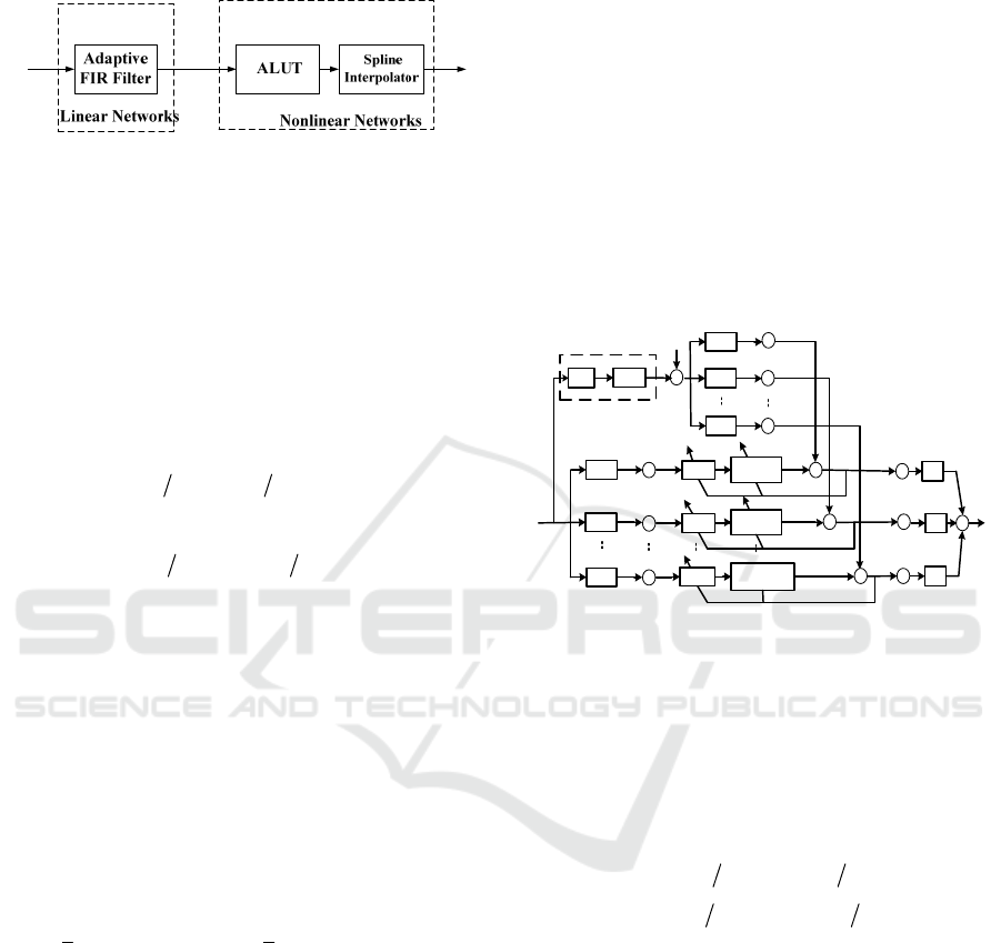
The block diagram of a SAF is shown in Fig.1,

which consists of an adaptive finite impulse respo-

nse (FIR) filter followed by a nonlinear network. In

the nonlinear network, the spline interpolater,

connected behind the adaptive LUT, determines the

number and the spacing of control points (knots)

contained in the LUT.

The input of the SAF at time n is

()

n , ()

represents the output of the linear networks which is

given by

Liu, C., Liu, X., Zhang, Z. and Tang, X.

Nonlinear Subband Spline Adaptive Filter.

In 3rd International Conference on Electromechanical Control Technology and Transportation (ICECTT 2018), pages 163-167

ISBN: 978-989-758-312-4

163

() ()(),

nnn= wx (1)

()

Figure 1: Block diagram of SAF.

where

01 1

() [ , , , ]

nww w

−

=w L represents the weight

vector of the FIR filter with length

, and

[(),( 1), ,))]((1

sn nns snB−−+=x L is the input vector

of the linear network.

With reference to the spline interpolation scheme

(Guarnieri, 1999), the output of the whole system

()yn and ()

n can be related by a local polynomial

function

()

, which depends on the span index i

and the local parameter

u . The two parameters are

defined as follows

() () ,

usnxsnx=Δ− Δ

⎢⎥

⎣⎦

(2)

() ( 1)2,

isnxQ=Δ+−

⎢⎥

⎣⎦

(3)

where

Δ is the uniform space between two control

points for the function

()

, Q is the total number

of control point and

⋅

⎢⎥

⎣⎦

denotes the floor operator.

The output of the whole system can be expressed as

() ( ) ,

in n in

yn u==φ uCq

(4)

where

C is the 44× spline basis matrix if the three-

order spline function is used. Two suitable types of

spline basis are B-spline and Catmull-Rom (CR)

spline (

Scarpiniti, 2013) which are given by

13 31 13 31

3 630 2 54-1

30 30 10 1 0

1410 0200

BCR

−− −−

⎡⎤⎡ ⎤

⎢⎥⎢ ⎥

−−

⎢⎥⎢ ⎥

= =

⎢⎥⎢ ⎥

−−

⎢⎥⎢ ⎥

⎣⎦⎣ ⎦

， (5)

where

[, ,,1]

nnn

uuu=u ,

,123

[, , , ]

in i i i i

qq q q

++ +

=q is the

control point vector and superscript

()

⋅ denotes

transposition.

3 SUBBAND SPLINE ADAPTIVE

FILTER (SSAF)

Fig.2 shows the block diagram of the proposed

SSAF.

()Φ  denotes the unknown nonlinear system

which generates the desired signal

[

]

)(()d

nn = Φ

()vn , where ()

n is the system input. ()vn is the

background noise, assumed to be zero mean ,and

independent of

()

n , its variance is

. The input

signal

()

and desired signal

()dn

are partitioned

into

subband signals

()

and

()

via the

analysis filters

()

Hz, 0,1, , 1.mM=−L The subband

signals,

()

dn and ()

n are critically decimated to

a lower sampling rate commensurate with their

bandwidth. We use the variable

n to index the

original sequences, and

k to index the decimated

sequence for all subband signals. The decimated

output for the

thm subband filter can be computed as

()dn

()vn

()Hz

()

−

()dk

()dn

()dk

()

−

()

()Hz

()

−

()

−

()

()xk

()

−

()kw

()yk

()ek

()yk

()

−

()ek

()

−

()Fz

()

−

()en

()

−

()en

0, 0,

(, )

()Sn

1, 1,

(, )

()

−

1, 1,

(, )

Mk Mk

−

−−i

()

−

()Φ



(, )xqφ



()dn

()

−

M↓

()kw

M↑

Figure 2: Block diagram of SSAF.

,,,

() ( )= ,

mimkmkik

yk u= φ uCq (6)

where

[,,,1]

mk mk mkmk

uuu=u

,(1)(2)

[,=, ,

mmm m

ik i i i

qq q

(3)

]

represents the

thm

subband control

point vector at the decimated time

. The

corresponding subband local parameter and subband

span index

i are defined as

() () ,

mkmmmm

uskxskx=Δ− Δ

⎢⎥

⎣⎦

(7)

() ( 1)2,

mm m m

iskx Q=Δ+−

⎢⎥

⎣⎦

(8)

where

is the total number of the control points

for the

thm

subband LUT and

Δ is the uniform

space, which can be selected to different values for

0,1, , 1.mM=−L

()

k is the output of the

thm

subband linear combiner which is given by

() () (),

mmm

kkk= wx (9)

where

,0 ,1 , 1

[(),(),,((]))

mmmmB

wkwk w kk

−

=w L

denotes

the weight vector of the subband FIR filter with

length

( ) [ ( ), ( 1), , ( 1)]

mm mm

ksksk skB−−+=s L

the subband input vector.

The subband output error can be expressed as

ICECTT 2018 - 3rd International Conference on Electromechanical Control Technology and Transportation

164

() () ()

=() ( ),

mmm

mimk

ek dk yk

dk u

=−

−

(10)

It is realized that the adaptation in each subband

is carried out independently as shown in Fig.2.

Therefore, the updating equations of the linear and

nonlinear networks for each subband can be derived

by minimizing the cost function

()

mmkik

{

}

=()

Ee k , where

{

}

E 

is the expectation

operator. For analytical simplicity, using the

instantaneous error instead of the expectation, we

get

()

,= 0,1,,1,

mmkik m

ekm M

() = −wq L (11)

and taking the partial derivative

()

mmkik

wq with

respect to

,mk

, we have

()

=()(),

mmkik

imk

mk mk m

mimkm

usk

ek u k

∂

− ()

∂∂∂

∂

′

− ()

φ x

(12)

where

()

imk

′

is the partial derivative of the local

activation function for the

thm subband,

()

imk

′

mk i k

uCq

,,,

[3 ,2 ,1,0]

mkmk

uu=u

, so the updating

equation of the linear networks for each subband can

be given as

(1)=() (),

mm mmkikm

kkek k

++ ()

ww uCqx

(13)

where

is the step-size for the linear network

adaptation.

For the subband nonlinear networks, the

derivative calculation of

()

mmkik

wq to

can

be defined by

()

=2 2() ,

mmkik

imk

mmmk

ik ik

ek ek

∂

− () =−

∂∂

(14)

The updating equation of the nonlinear networks

for each subband can be written as

,1 , q ,

=(),

ik ik m mk

+qq Cu (15)

4 COMPUTATIONAL

COMPLEXITY

Note that (13) and (15) are the updating equations of

the LMS algorithm for the proposed SSAF. For each

iteration, only four control points for each subband

are changed because of the local behavior of the

spline function. This leads to a large computational

savings. The computational complexity of the pro-

posed SSAF solution is mainly evaluated in terms of

the number of multiplications per sample.

Note that

for each subband , the control points of the LUT and

the weights of the FIR filter are updated every M

samples due to the critical sampling. Considering

that there are M subband signals par-ticipating in the

adaptation, it requires 2B+1 multi-plications for the

linear updating equation (13) and B multiplications

for the output estimation of the linear network. For

the spline output calculation and adap-tation, like the

conventional SAF (Scarpiniti, 2013), we take into

account of the repetitive appearance of the terms

Cq ,

in (6), (13) and (15), it only needs 4K

multiplications by the date reuse of the past

computations, where K

(less than 16) is the

constant which can be defined with reference to the

implementation spline structure in (Guarnieri, 1999).

In addition, the subband input signal and desired

signal partition needs

multiplications, where

is the length of the analysis and synthesis filters.

For error signal synthesis, it needs

multiplications. Therefore, compared with the SAF

scheme, the proposed one only requires extra

multiplications for the subband signal analysis and

synthesis.

5 EXPERIMENTAL RESULTS

To confirm the performance of the proposed scheme

in this paper, we present the experimental results of

the proposed scheme for the nonlinear system

identification. All the following results are obtained

by averaging over 50 Monte Carlo trials. The

performance is measured by use of mean square

error (MSE) defined as

10log [ ( )]en

. The input

signal is generated by the process

() ( 1) 1 ()

nxn n

ωωβ

=−+− ， (16)

where

()n

is the White Gaussian noise signal with

zero mean and unitary variance, the parameter

selected in the range

[0, 0.95] , which interprets the

degree of correlation for the adjacent samples. The

FIR filter coefficients for the SAF and SSAF model

Nonlinear Subband Spline Adaptive Filter

165

are initialized as

-1

=[ ,0,...,0]

w with length

and

<≤, while the spline model is initially set to a

straight line with a unitary slope. For convenience,

only B-spline basis is applied in the simulations,

however, the similar results can also be achieved

using the CR-spline basis.

5.1 Experimental 1

The unknown system model

()Φ 

is the Wiener

spline model which comprises a FIR filter

[0.6, 0.4,0.25, 0.15,0=.1]

−−w and a nonlinear spline

function represented by a 23 control points length

LUT

q ,

Δ and

are set to 0.2 and

q is

defined by

[ 2.2, 2.0, 1.8, 1.6, 1.4, 1.2, 1.0, 0.8, 0.91,

0.4, 0.2, 0.05,0, 0.4,0.58,1.0,1.0,1.2,1.4,1.6,1,8, 2.0, 2.2],

=−−−−−−−−−

− − −

(17)

For signal partitioning in this experiment, The

cosine-modulated filter banks with subband number

2, 4,K = and 8 are used and the prototype filters’

length of analysis filter increases with the number of

subband, the prototype filters’ length ,

P , are 32 , 64

and 128 for

2, 4,M = and 8 correspondently. The

default values

0.5

= , 0.1

= , and 5B = are emp-

loyed and 10000 samples are used. An independent

White Gaussian noise signal,

()vn , is added to the

output of the unknown system, with 23-dB, 26-dB,

30dB signal to noise ratio (SNR) for

2, 4,8M =

respectively. The step sizes are selected to ensure

that the conventional SAF and the SSAF obtain the

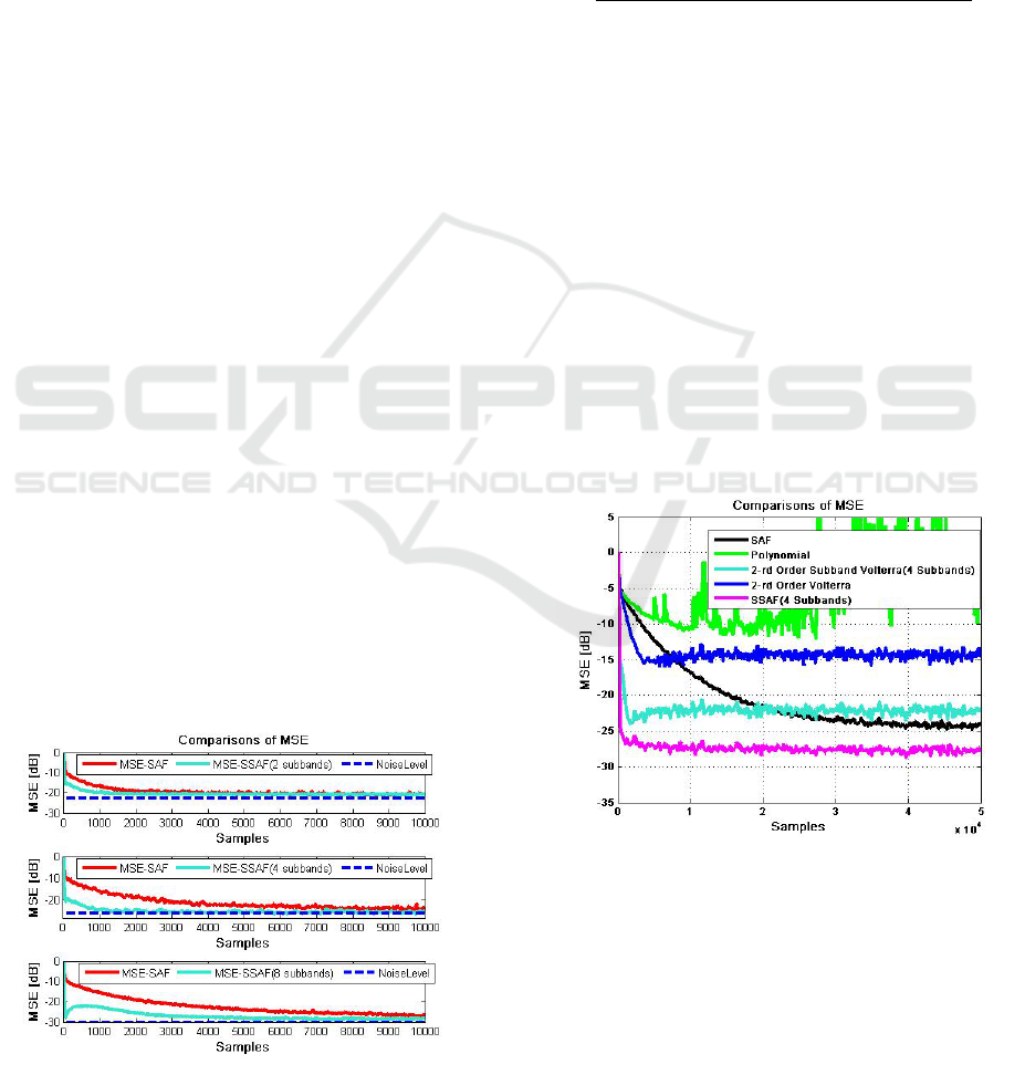
similar steady-state MSE. The performances of the

SAF and proposed SSAF are compared for the diff-

erent numbers of subband in Fig.3. It can be seen

that the proposed SSAF supplies the faster conver-

gence rate than the SAF. This is due to the

decorrelating properties of the subband scheme for

colored input signals.

Figure 3: MSE curves of the SAF and SSAF.

5.2 Experimental 2

In the second experiment, we compare the MSE

performance of the polynomial model (Stenger,

2000), 2-rd order Volterra model (Kuech, 2002), 2-

rd order subband Volterra model (Burton, 2009),

SAF model (Scarpiniti, 2013) and proposed SSAF

model. The unknown system to be identified

()Φ



consists of two blocks, the first one is the 3-order

IIR filter

123

12 3

0.0154 0.046 0.0462 0.0154

() ,

1 1.99 1.572 0.4583

zzz

zz z

−−−

−− −

++ +

−+ −

(18)

and the second block nonlinearity

( ) sin( [ ]).yn xn= (19)

The number of subband is set to 4 for the SSAF

and 2-rd order subband Volterra model. The cosine-

modulated filter banks with subband number

are used and the prototype filters’ length is selected

to 64. The step sizes are set to

= =0.01

μμ

for both

the HSAF and the SSAF, step size =0.001

is used

for the polynomial model and the step size is set to

0.01 for the 2-rd order Volterra and 2-rd order

subband Volterra model. The signal to noise ratio is

30SNR dB= . The default values 0.6

= , 0.1

= ,

==0.2

xxΔΔ and 15B = are employed and 50000

samples are used. A comparison of the MSE learn-

ing curves is reported in Fig. 4, it can be clearly

noted that the robustness of the proposed SSAF.

Figure 4: Comparison MSE of the different models in

experiment 2.

ICECTT 2018 - 3rd International Conference on Electromechanical Control Technology and Transportation

166

5.3 Experimental 3

The third experiment aims to test the effectiveness

of the proposed structure in case of a high degree of

nonlinearity. The unknown system in system ident-

ification

()Φ  comprises three blocks. The first and

the last blocks are IIR filters whose transfer function

can be written as

0.2851 0.5704 0.2851

()

1 0.1024 0.4475

0.2025 0.2880 0.2025

1 0.6591 0.1498

−−

⎛⎞

⎜⎟

−+

⎝⎠

⎛⎞

⎜⎟

−+

⎝⎠

(20)

0.2025 0.2880 0.2025

()

1 1.01 0.5861

0.2025 0.2880 0.2025

1 0.6591 0.1498

−−

⎛⎞

⎜⎟

−+

⎝⎠

⎛⎞

⎜⎟

−+

⎝⎠

(21)

and the nonlinear portion of this model is expressed

2()

() .

1()

(22)

It is noted that this model is capable of

describing the behavior model of the radio frequency

amplifier for satellite communications (Scarpiniti,

2013). For both the SAF and the SSAF, linear filter

length

B is set to 15. The parameter

is set to 0.2.

All the other parameters are set to similar values as

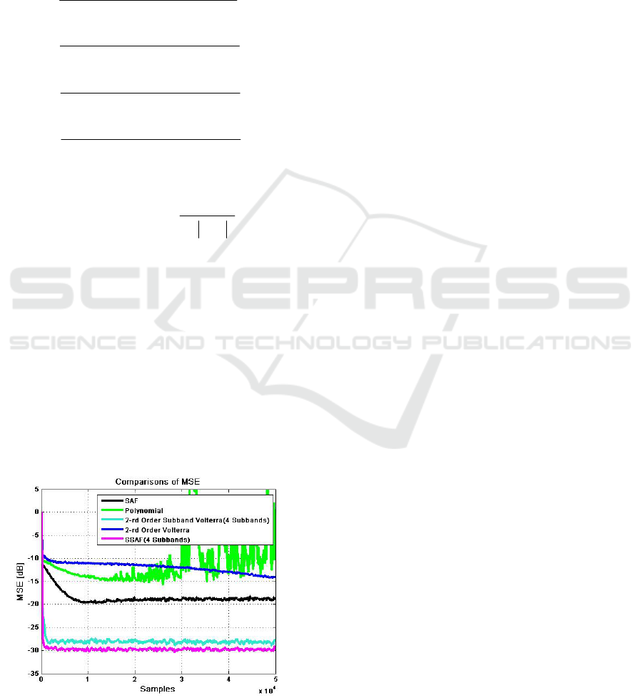
in Experimental 2. Fig. 5 shows that the comparison

of the MSE learning curves for several models, it is

clear in this case that the deteriorating performance

of the Polynomial model and the 2-rd order Volterra

model, verifying that these two models only cope

with the case of mile nonlinearity. Furthermore, the

proposed SSAF obtains the best convergence

performance with respect to other models.

Figure 5: Comparison MSE of the different models in

experiment 3.

6 CONCLUSIONS

In this paper, a novel SSAF structure for nonlinear

system identification is presented. It consists of a

series of subband nonlinear filters, the adaptation of

these subband filters is carried out independently.

The computational complexity is analyzed based on

the LMS algorithm. Some experimental results in

the context of the nonlinear system identification

show the effectiveness of the proposed structure.

ACKNOWLEDGEMENTS

This research was supported by the National Natural

Science Foundation of China (61501119).

REFERENCES

Mathews V.J., Sicuranza G.L., 2000. Polynomial Signal

Processing.

John Wiley & Sons, Hoboken, New

Jersey.

Schetzen M., 1980.

The Volterra and Wiener Theories of

Nonlinear Systems

, John Wiley & Sons, New York,.

Haykin S., 2009.

Neural Networks and Learning Machines,

Pearson Publishing, 2

ed.

Giri F., Bai E.W., (Eds.), 2010.

Block-Oriented Nonlinear

System Identification,

Springer-Verlag, Berlin.

Scarpiniti M., Conniniello D., Parisi R., Uncini A., 2013.

Nonlinear spline adaptive filtering, Signal Proce-ssing

93(4) 772–783.

Scarpiniti M., Conniniello D., Parisi R., Uncini A., 2014.

Hammerstein uniform cubic spline adaptive filtering:

Learning and convergence properties

, Si-gnal

Processing 100(4) 112–123.

Scarpiniti M., Conniniello D., Parisi R., Uncini A., 2015.

Novel cascade spline architectures for the id-

entification of nonlinear systems

, IEEE Tran-sanctions

on Circuits and Systems-I: regular papares 62(7) 1825-

1835.

Guarnieri S., Piazza F., Uncini A., 1999.

Multilayer

feedforward networks with adaptive spline activation

function

, IEEE Transanctions on Neural Networks,

10(3) 672-683.

Burton T. G., Goubran R.A., 2009. Beaucoup F.,

Non-

linear system identification using a sub-band adaptive

Volterra filter

, IEEE Transanctions on Instrumentation

and Measurement, 58(5) 1389-1397.

Stenger S., Kellerman W., 2000.

Adaptation of a

memoryless preprocessor for nonlinear acoustic echo

cancelling

, Signal Processing, 80(9) 1747–1760.

Kuech F., Kellerman W., 2002.

Nonlinear line echo

cancellation using a simplified second order Volterra

filter

, in Proceedings of the ICASSP, vol. 2, Orlando,

Flo-rida, 1117–1120.

Nonlinear Subband Spline Adaptive Filter

167