
Revisiting Population Structure and Particle Swarm Performance
Carlos M. Fernandes
1
, Nuno Fachada
1,2
, Juan L. J. Laredo
3
, Juan Julian Merelo
4
,
Pedro A. Castillo
4
and Agostinho Rosa
1
1
LARSyS: Laboratory for Robotics and Systems in Engineering and Science, University of Lisbon, Lisbon, Portugal
2
HEI-LAB - Digital Human-Environment and Interactions Labs, Universidade Lusófona, Lisbon, Portugal
3
LITIS, University of Le Havre, Le Havre, France
4
Departamento de Arquitectura y Tecnología de Computadores, University of Granada, Granada, Spain
Keywords: Particle Swarm Optimization, Population Structure, Regular Graphs, Random Graphs.
Abstract: Population structure strongly affects the dynamic behavior and performance of the particle swarm
optimization (PSO) algorithm. Most of PSOs use one of two simple sociometric principles for defining the
structure. One connects all the members of the swarm to one another. This strategy is often called gbest and
results in a connectivity degree =, where is the population size. The other connects the population in
a ring with =3. Between these upper and lower bounds there are a vast number of strategies that can be
explored for enhancing the performance and adaptability of the algorithm. This paper investigates the
convergence speed, accuracy, robustness and scalability of PSOs structured by regular and random graphs
with 3≤≤. The main conclusion is that regular and random graphs with the same averaged
connectivity may result in significantly different performance, namely when is low.
1 INTRODUCTION
Particle Swarm Optimization (PSO) is a collective
intelligence model for optimization and learning
(Kennedy and Eberhart, 1995) that uses a set of
position vectors (called particles) to represent
candidate solutions to a specific problem. These
particles move through the fitness landscape of a
specified target-problem following a set of behavioral
equations that define their velocity at each time step.
After updating the velocity and position of each
particle as well as to the global and local information
about the search, the fitness of every particle is
computed. The process repeats until a stop criterion is
met.
Information on the current and previous state of
the search flows through the graph that connects the
particles, informing them on the best solutions found
by their neighbors. The graph can be of any form and
affects the balance between exploration and
exploitation and consequently the convergence speed
and accuracy of the algorithm. The reason why
particles are interconnected is the core of the
algorithm: particles communicate so that they acquire
information on the regions explored by other
particles. In fact, it has been claimed that the
uniqueness of the PSO algorithm lies in the inter-
actions of the particles (Kennedy and Mendes, 2002).
As stated, the population can be structured on any
possible topology, from sparse to dense (or even fully
connected) graphs), with different levels of
connectivity and clustering. The classical and most
used population structures are the lbest with ring
topology (which connects the individuals to a local
neighborhood) and the gbest (in which each particle is
connected to every other individual). These topologies
are well-studied and the major conclusions are that
gbest is fast but is frequently trapped in local optima,
while lbest is slower but converges more often to the
neighborhood of the global optima.
Studies have tried to understand what makes a
good structure. For instance, Kennedy and Mendes
(Kennedy and Mendes, 2002) investigated several
types of topologies and recommend the use of a lattice
with von Neumann neighborhood (which results in a
connectivity degree between that of lbest and gbest).
Others, like (Parsopoulos and Vrahatis, 2005), have
tried to design networks that hold the best traits given
by each structure.
This paper revisits the study in (Kennedy and
Mendes, 2002). Although the authors provided
significant insight on the relationship between
population structure and PSO performance, the study
248
Fernandes, C., Fachada, N., Laredo, J., Merelo, J., Castillo, P. and Rosa, A.
Revisiting Population Structure and Particle Swarm Performance.
DOI: 10.5220/0006959502480254
In Proceedings of the 10th International Joint Conference on Computational Intelligence (IJCCI 2018), pages 248-254
ISBN: 978-989-758-327-8
Copyright © 2018 by SCITEPRESS – Science and Technology Publications, Lda. All rights reserved

was mainly dedicated to random topologies and few
levels of connectivity were inspected. Some aspects
of the research subject that were overlooked are now
worth investigating, namely the importance of graph
regularity and the performance of regular and random
graphs with the same level of connectivity. This paper
investigates and compares the convergence speed,
accuracy, robustness and scalability of PSOs
structured by regular and random graphs with
different connectivity. Finally, the topologies were
not only tested on standard fixed-parameters PSOs,
but also on a PSO with time-varying parameters.
The present work is organized as follows. Section
2 gives a background review on PSO and population
structures. Section 3 describes the experiment setup
and Section 4 discusses the results. Finally, Section 5
concludes the paper and outlines future lines of
research.
2 BACKGROUND REVIEW
PSO is described by a simple set of equations that
define the velocity and position of each particle. The
position vector of the i-th particle is given by
=
(
,
,
,
,…
,
), where is the dimension of the
search space. The velocity is given by
=
(
,
,
,
,…
,
). The particles are evaluated with a
fitness function (
) and then their positions and
velocities are updated by:
,
(
)
=
,
(
−1
)
+
,
−
,
(−1)
+
,
−
,
(−1)
(1)
,
(
)
=
,
(
−1
)
+
,
(
)
(2)
were
is the best solution found so far by particle
and
is the best solution found so far by the
neighborhood. Parameters
and
are vectors of
random values uniformly distributed in the range
[0,1] and
and
are acceleration coefficients.
In order to prevent particles from moving out of
the limits of the search space, the positions
,
(
)
of
the particles are limited by constants that, in general,
correspond to the domain of the problem:
,
(
)
∊
[
−,
. Velocity may also be limited
within a range in order to prevent the explosion of the
velocity vector:
,
(
)
∊
[
−,
. Usually,
=.
Although the classical PSO can be very efficient
on numerical optimization, it requires a proper
balance between local and global search, as it often
gets trapped in local optima. In order to achieve a
better balancing mechanism, (Shi and Eberhart, 1998)
added the inertia weight for fine-tuning the local
and global search abilities of the algorithm.
By adjusting (usually within the range [0, 1.0])
together with the constants
and
, it is possible to
balance exploration and exploitation abilities of the
PSO. The modified velocity equation is:
,
(
)
=.
,
(
−1
)
+
,
−
,
(−1)
+
,
−
,
(−1)
(3)
The neighborhood of the particle defines in each
time-step the value of
and is a key factor for the
performance of the algorithm. Most of the PSOs use
one of two simple principles for defining the
neighborhood network. One connects all the members
of the swarm to one another and is called gbest, where
g stands for global. The degree of connectivity of
gbest is =, where n is the number of particles.
The other typical configuration, called lbest (l stands
for local), creates a neighborhood that comprises the
particle itself and its nearest neighbors. The most
common lbest topology is the ring structure.
As stated above, the topology of the population
affects the performance of the PSO and the
configuration must be chosen according to the target-
problem and the performance requirements (i.e., the
acceptable compromise between convergence speed
and accuracy). Since all the particles are connected to
every other and information spreads easily through
the network, the gbest topology usually converges fast
but unreliably (it often converges to local optima).
The lbest converges slower than gbest because
average path length of the network is higher and
information spreads slower, but, for the same reason,
it is also less prone to converge prematurely to local
optima.
In-between the ring structure with =3 and the
gbest with = there are several possibilities, each
one with its advantages and drawbacks. Very often it
is not possible to choose beforehand the optimal or
near-optimal configuration: for instance, when the
properties of the problem are unknown or the time
requirements do not permit preliminary tests.
Therefore, substantial research efforts have been
dedicated to PSO’s population structures.
In 2002, (Kennedy and Mendes, 2002) tested
several types of structures, including lbest, gbest and
von Neumann configurations. They also tested
populations arranged in graphs that were randomly
generated and optimized to meet some criteria. The
authors concluded that when the configurations were
ranked by the performance at 1000 iterations the
Revisiting Population Structure and Particle Swarm Performance
249

structures with k = 5 perform better, but when ranked
according to the number of iterations needed to meet
the criteria, configurations with higher degree of
connectivity perform better. These results are
consistent with the premise that low connectivity
favors robustness, while higher connectivity favors
convergence speed (at the expense of reliability).
The unified PSO (UPSO) (Parsopoulos and
Vrahatis, 2005) combines gbest and lbest
configurations. Equation 1 is modified in order to
include a term with
and a term with
while a
parameter balances the weight of each term. The
authors argue that the proposed scheme exploits the
good properties of gbest and lbest.
(Peram et al., 2003) proposed the fitness–distance-
ratio-based PSO (FDR-PSO). The algorithm defines
the neighborhood of a particle as its closest particles
in the population (measured in Euclidean distance). A
selective scheme is also included: the particle selects
near particles that have also visited a position of
higher fitness. The authors claim that FDR-PSO
performs better than the standard PSO on several test
functions. However, FDR-PSO is compared only to
the gbest configuration. Recently, (Ni et al., 2014)
proposed a dynamic probabilistic PSO. The authors
generate random topologies for the PSO that they use
at different stages of the search.
3 EXPERIMENTAL SETUP
First, several regular graphs have been constructed
using the following procedure: starting from a ring
structure with =3 the degree is increased by
linking each individual to its neighbors’ neighbors,
thus creating a set of regular graphs with =
{3,5,7,9,11…,}, as exemplified in Figure 1 for a
swarm with 8 particles (the configuration is easily
generalized to other population sizes).
=3 =5 =
Figure 1: Regular graphs with population size =.
For the experiments discussed in this paper, PSOs
with population size =33 have been used and
regular graphs with ={3,5,7,9,13,17,25,33}
were constructed. Please note that the regular graph
with =33 corresponds to the gbest topology. Then,
random graphs with 33, 66, 99, 132, 198, 264 and 396
bi-directional edges were also generated,
corresponding to an average level of connectivity
′={3,5,7,9,13,17,25,33}. Again, the random
graph with ′=33 is equivalent to the gbest
structure.
The acceleration coefficients of the fixed-
parameters PSO were set to 1.49618 and the inertia
weight is 0.729844 (Rada-Vilela et al., 2013). An
alternative approach to fixed parameter tuning is to let
the values change during the run, according to
deterministic or adaptive rules. (Shi and Eberhart,
1998) proposed a linearly time-varying inertia weight.
The variation rule is given by Equation (4).
()=
(
−
)
×
(max_−)
max_
+
(4)
where is the current iteration, _ is the
maximum number of iterations,
the inertia weigh
initial value and
its final value.
Later, (Ratnaweera et al., 2004) proposed to
improve Shi and Eberhart’s PSO with time-varying
inertia weight (PSO-TVIW) using a similar concept
applied to the acceleration coefficients. In the PSO
with time-varying acceleration coefficients PSO
(PSO-TVAC) the parameters
and
change during
the run according to the following equations:
=
−
×
max_
+
(5)
=
−
×
max_
+
(6)
where
,
,
,
are the acceleration coefficients
initial and final values. For the experiments with
PSO-TVAC in the following section, parameters
and
were set to 0.9 and 0.4, the acceleration
coefficient
initial and final values were set to 2.5
and 0.5 and
ranges from 0.5 to 2.5, as suggested in
(Ratnaweera et al, 2004).
Table 1: Benchmark functions.
mathematical
representation
search
range/
initialization
stop
criterion
sphere
f
1
(
)
=
(−100,100
)
(50,100)
0.000001
quadric
f
2
(
)
=
(−100,100
)
(50,100)
0.01
IJCCI 2018 - 10th International Joint Conference on Computational Intelligence
250

Table 1: Benchmark functions (cont.).
mathematical
representation
search
range/
initialization
stop
criterion
hyper
ellipsoid
f
3
(
)
=
(−100,100
)
(50,100)
0.
000001
rastrigin
f
4
(
)
=
(
−10cos
(
2
)
+10
)
(−10,10)
(2.56,5.12)
100
griewank
f
5
(
)
=1+
1
4000
−
cos
√
(−600,600
)
(300,600)
0.05
weierstrass
f
6
(
)
=
2
(
+0.5
)
−
[
(
2
∙0.5
)
,
=0.5,=3,=20
(−0.5,0.5)
(−0.5,0.2)
0.01
ackley
f
7
(
)
=−20
−0.2
1
−
1
cos
(
2
)
+20+
(−32.768,3
2
(2.56,5.12)
0.01
shifted
quadric
with noise
f
8
(
)
=
∗
(
1+0.4
|
(
0,1
)|)
,
=− ,
=
[
,..
:
(−100,100
)
(50,100)
0.01
rotated
griewank
f
9
(
)
=1+
∑
−
∏
cos
√
,
=,
M:ortoghonal matrix
(−600,600
)
(300,600)
0.05
Figure 2: Success rates (50 runs). Regular graphs. Problem
dimension =30. Standard PSO with fixed-parameters.
is defined as usual by the domain’s upper
limit and =. A total of 50 runs for
each experiment were performed. Nine benchmark
problems were used. Functions f
1
-f
3
are unimodal; f
4
-f
7
are multimodal; f
8
is the shifted f
2
with noise and f
9
the
rotated f
5
(f
8
global optimum and f
9
matrix were taken
from CEC2005 benchmark). Asymmetrical
initialization is used (initialization range for each
function is given in Table 1).
Two sets of experiments were conducted. First,
the algorithms were run for a specific amount of
function evaluations (330000 for
and
, 660000
for the remaining). The best solution was recorded
after each run. Each algorithm has been executed 50
times in each function. Statistical measures were
taken over those 50 runs. In the second set of
experiments the algorithms were run for 660000
evaluations or until reaching function-specific stop
criteria (given in Table 1). A success measure is
defined as the number of runs in which an algorithm
attains the criterion. Again, each one has been
executed 50 times in each function. This setup is as in
(Kennedy and Mendes, 2002)0.
The algorithms discussed in this paper are
available in the OpenPSO package, which offers an
efficient, modular and multicore-aware framework for
experimenting with different PSO approaches. The
package is implemented in C99, and transparently
parallelized with OpenMP (Dagum and Menon,
1998). The library components can be interfaced with
other programs and programming languages, making
OpenPSO a flexible and adaptable framework for
PSO research. The source code is at
https://github.com/laseeb/openpso.
4 RESULTS AND DISCUSSION
The main objectives of the experiments are to
examine how fixed-parameters PSOs perform with
different levels of connectivity and investigate if the
relative performance varies with problem dimension.
Figure 3: Evaluations required to meet criteria: median
values (50 runs). Regular graphs. Problem dimension =
30. Fixed-parameters PSO.
0
10
20
30
40
50
k = 3 k = 5 k = 7 k = 9 k = 13 k = 17 k = 25 k = 33
f1
f2
f3
f4
f5
f6
f7
f8
f9
0
20000
40000
60000
80000
100000
120000
140000
160000
180000
200000
k = 3 k = 5 k = 7 k = 9 k = 13k = 17k = 25k = 33
f1
f2
f3
f4
f5
f6
f7
f8
f9
Revisiting Population Structure and Particle Swarm Performance
251

Then, study the differences between the performance
of PSOs with regular and random graphs. Finally,
confirm if the same general conclusions apply to
time-varying strategies for parameter setting.
4.1 Regular Graphs
The first experiment compares the success rates,
convergence speed and accuracy (best solutions) of
fixed-parameters PSO on regular graphs. Problem
dimension is =30. Figure 2 shows the success
rates of the algorithm on each function with each
regular graph. In general, better success rates are
attained with lower connectivity, but there are two
exceptions: functions
and
. However, these
results are in general terms in accordance with those
in (Kennedy and Mendes, 2002): configurations with
lower connectivity attain better success rates.
Figure 3 represents the median values of the
evaluations required to meet the stop criteria. Clearly,
the convergence speed increases with connectivity
degree . These findings are in different from those in
(Kennedy and Mendes, 2002), where it is reported
that the configurations with =5 (from a set with
=3, =5 and =10 graphs) required less
evaluations to meet the stop criteria. However, those
experiments were conducted under different
conditions, like population size and, namely, graph
types: here, we are testing PSO on regular graphs with
varying size.
Table 2 shows the median values of the best
fitness attained in each of the 50 runs, for each
function and each graph. The best graphs according
Table 2: Best fitness. Median values. Regular graphs.
Problem dimension D = 30. Fixed-parameters PSO.
=3 =5 =7 =9 =13 =17 =25=33
f
1
1.96e-89 7.85e-90 3.93e-90 1.96e-90 1.96e-90 0.00e00 0.00e00 3.93e-90
f
2
7.59e-13 1.04e-20 2.49E-25 4.41e-29 3.03e-34 6.04e-37 1.00e+04 2.00e+04
f
3
1.67e-88 3.34e-89 5.89e-90 1.96e-90 0.00e00 0.00e00 0.00e00 4.50e+04
f
4
1.18e+02 8.71e+01 8.31e+01 7.26e+01 8.31e+01 8.66e+01 8.71e+01 1.28e+02
f
5
0.00e+00 0.00e+00 0.00e+00 0.00e+00 1.11e-02 7.40e-03 9.86e-03 6.85e-02
f
6
0.00e+00 0.00e+00 6.17e-03 6.78e-02 1.02e+00 2.03e+00 4.33e+00 6.03e+00
f
7
7.55e-15 7.55e-15 7.55e-15 7.55e-15 7.55e-15 7.55e-15 1.25e+00 1.90e+00
f
8
2.02e+02 1.32e+01 9.23e-01 3.43e-01 4.98e+03 9.30e+03 2.86e+04 4.74e+04
f
9
0.00e00 0.00e00 0.00e00 8.63e-03 1.23e-02 1.72e-02 5.09e-01 4.25e+01
Figure 4: Success rates (50 runs). Regular graphs. Problem
dimension =10. Standard PSO with fixed-parameters.
to the accuracy criteria depend on the type of
function. For unimodal functions (
,
,
and
)
best results are attained with highly connected graphs,
while multimodal functions require graphs with lower
connectivity.
In (Kennedy and Mendes, 2002), configurations
with =5 yielded the best fitness values and
required less evaluations to meet the criteria, while
=3 had the best success rates. The results in this
paper, although they do not necessarily contradict the
experiments in (Kennedy and Mendes, 2002) (which
were conducted under different conditions), provide
some more insight on the performance of PSO
populations with different connectivity levels.
4.2 Problem Dimension
The next test investigates the behavior of the
algorithm with different problem dimension. For that
purpose, was set to =10 and =50. The
algorithms were tested as in the previous experiment.
Figure 4 and Figure 5 show the success rates for
=10 and =50 respectively. Changing the
problem dimension does affect the general behavior
of the PSO on regular graphs with different
connectivity levels: lower graphs yield better
success rates for =10 and =50 (the most
notorious exception is
when =50). Some
functions behave differently, namely
and
(Griewank and rotated Griewank), for which the
success rates tend to increase with . However, the
overall performance scales as expected, as seen in
Figure 6, which depicts the percentage of successful
runs of each type of graph for each averaged over
the whole set of functions.
0
10
20
30
40
50
k = 3 k = 5 k = 7 k = 9 k = 13 k = 17 k = 25 k = 33
f1
f2
f3
f4
f5
f6
f7
IJCCI 2018 - 10th International Joint Conference on Computational Intelligence
252
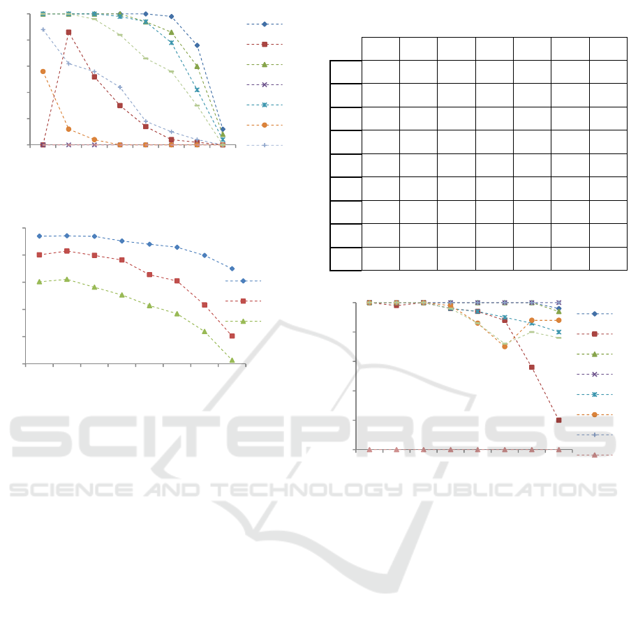
Figure 5: Success rates (50 runs). Regular graphs. Problem
dimension =50. Standard PSO with fixed-parameters.
Figure 6: Percentage of successful runs averaged over the
set of functions. Regular graphs. Fixed-parameters PSO.
As for the convergence speed and accuracy, the
results lead to the same conclusions as in Section 4.1
for =30: convergence speed for =10 and =
50 increases with and accuracy depends on the type
of function: unimodal are better tackled with highly
connected graphs while multimodal problems require
graphs with lower connectivity.
4.3 Time-varying Parameters
A final experiment implemented and tested the PSO-
TVAC on the set of regular graphs. Success rates are
shown in
Figure 7. PSO-TVAC is able to meet the criteria in
every function (except
) with =3 and =7. It
also improves the performance of standard PSO on
several functions for higher values. On the other
hand, it is significantly slower than the standard PSO
on every function and every .
Mann-Whitney tests were performed to compare
the distributions of the number of evaluations to meet
criteria of each graph in each function confirming that
the PSO is significantly faster than PSO-TVAC in
every function and . Comparing Figure 8 and Figure
3 gives an overall idea on the magnitude of the
differences in convergence speed.
Table 3: Best fitness. Median values. Random graphs.
Problem dimension D = 30. Fixed-parameters PSO.
′=3 ′=5 ′=7 ′=9 ′=13 ′=17 ′=25
f
1
1.57e-89 5.89e-90 3.93e-90 1.96e-90 1.96e-90 0.00e+00 0.00e+00
f
2
5.00e+03 6.39e-26 3.02e-29 1.13e-31 6.85e-35 6.65e-38 1.00e+04
f
3
1.21e-88 1.08e-89 5.89e-90 0.00e+00 0.00e+000.00e+000.00e+00
f
4
1.13e+027.56e+016.91e+01 7.91e+01 8.51e+01 8.31e+01 9.60e+01
f
5
1.23e-02 9.86e-03 3.70e-03 7.40e-03 7.40e-03 1.23e-02 9.86e-03
f
6
2.52e+00 1.51e-01 2.00e-01 7.52e-01 1.13e+00 1.92e+003.64e+00
f
7
1.78e+00 7.55e-15 7.55e-15 7.55e-15 7.55e-15 1.11e-14 1.16e+00
f
8
2.26e+043.16e+02 1.77e-01 3.45e+01 2.58e+02 1.33e+04 2.20e+04
f
9
3.31e-02 9.86e-03 9.86e-03 7.40e-03 2.22e-02 1.23e-02 5.20e-01
Figure 7: Success rates (50 runs). Regular graphs.
Problem dimension D = 30. PSO-TVAC.
5 CONCLUSIONS
This paper investigates the performance of PSOs
with regular and random structures. A set of regular
and random graphs with different levels of
connectivity were constructed and used as network
topologies for the algorithms. Success rates,
convergence speed, accuracy and scalability have
been investigated. Results show that the probability
of meeting the stop criteria (success rates) is higher
when the degree of connectivity is lower.
However, convergence speed increases with . As
for the accuracy, the experiments showed that best
results on unimodal functions are attained with
highly connected graphs while lower connectivity is
more suited for multimodal functions. The general
behavior maintains when varying the search space
dimension. Also, PSOs with fixed and time-varying
parameters behave similarly throughout the range of
regular graphs.
0
10
20
30
40
50
k = 3 k = 5 k = 7 k = 9 k = 13 k = 17 k = 25 k = 33
f1
f2
f3
f4
f5
f6
f7
0
0,2
0,4
0,6
0,8
1
k = 3 k = 5 k = 7 k = 9 k = 13 k = 17 k = 25 k = 33
D = 10
D = 30
D = 50
0
10
20
30
40
50
k = 3 k = 5 k = 7 k = 9 k = 13 k = 17 k = 25 k = 33
f1
f2
f3
f4
f5
f6
f7
f8
Revisiting Population Structure and Particle Swarm Performance
253

One of the most interesting results concerns the
comparison between regular and random graphs.
The experiments demonstrated that switching from a
regular to a random graph with the same level of
connectivity degrades PSO success rates and
accuracy when is low, while for higher the
results are similar. This is probably due to the high
variance of the average in graphs with low
connectivity but further investigation is required to
confirm this hypothesis.
Figure 8: Evaluations required to meet criteria: median
values (50 runs). Regular graphs. Problem dimension =
30. PSO-TVAC.
The analysis in this paper has been mainly
qualitative and supported by graphical depiction of
the results. In the future, the data will organized and
normalized in order to perform exhaustive statistical
tests that will hopefully give more insight on the
relationship between performance and population
structure and provide support to the conclusions and
hypothesis raised by this study. In addition, more
random graphs will be generated and tested, with
different standard deviation of and clustering
degree. Finally, the effect of dynamic structures in the
performance of PSO will be investigated.
ACKNOWLEDGEMENTS
First author wishes to thank FCT, Ministério da
Ciência e Tecnologia, his Fellowship
SFRH/BPD/111065/2015). This work was supported
by FCT PROJECT [UID/EEA/50009/2013].
REFERENCES
Dagum, L, Menon, R. 1998. OpenMP: an industry
standard API for shared-memory programming. IEEE
Computational Science and Engineering, 5(1), 46-55.
Kennedy, J, Eberhart, R. 1995. Particle swarm
optimization. In Proceedings of IEEE International
Conference on Neural Networks, Vol.4, 1942–1948.
Kennedy, J, Mendes, R. 2002. Population structure and
particle swarm performance. In Proceedings of the
IEEE World Congress on Evolutionary Computation,
1671–1676.
Ni, Q, Cao, C, Yin, X. 2014. A new dynamic probabilistic
Particle Swarm Optimization with dynamic random
population topology. In 2014 IEEE Congress on
Evolutionary Computation, 1321-1327.
Parsopoulos, K, Vrahatis, M. 2005. Unified particle swarm
optimization in dynamic environments. Lecture Notes
in Computer Science (LNCS), Vol. 3449, Springer,
590-599.
Peram, T, Veeramachaneni, K, Mohan, C. 2003. Fitness-
distance-ratio based particle swarm optimization. In
Proc. Swarm Intell. Symp., 174–181.
Rada-Vilela, J, Zhang, M, Seah, W. 2013. A performance
study on synchronous and asynchrounous updates in
particle swarm. Soft Computing, 17(6), 1019–1030.
Ratnaweera, A, Halgamuge, S, Watson, H. 2004. Self-
organizing hierarchical particle swarm optimizer with
time varying accelerating coefficients. IEEE
Transactions on Evolutionary Computation, 8(3),
240–255.
Shi, Y, Eberhart, R. 1998. A modified particle swarm
optimizer. In Proceedings of IEEE 1998 International
Conference on Evolutionary Computation, IEEE
Press, 69-73.
Shi, Y, Eberhart, R. 1999. Empirical study of particle
swarm optimization. In Proceedings of IEEE
International Congress on Evolutionary Computation,
vol. 3, 101–106.
0
50000
100000
150000
200000
250000
300000
k = 3 k = 5 k = 7 k = 9 k = 13 k = 17 k = 25 k = 33
f1
f2
f3
f4
f5
f6
f7
IJCCI 2018 - 10th International Joint Conference on Computational Intelligence
254
