LCA Histogram Distance for Rooted Labeled Caterpillars

Takuya Yoshino, Kohei Muraka and Kouichi Hirata

Kyushu Institute of Technology, Kawazu 680-4, Iizuka 820-8502, Japan

Keywords:

LCA Histogram Distance, Rooted Labeled Caterpillars, Path Histogram Distance, Complete Subtree

Histogram Distance.

Abstract:

An LCA histogram distance is an L

-distance between histograms consisting of triples of two nodes and their

least common ancestor (LCA) in two trees. In this paper, we show that the LCA histogram distance for cater-

pillars is always a metric, whereas that for trees is not. Then, we give experimental results for computing the

LCA histogram distance by comparing with the path histogram distance and the complete subtree histogram

distance for caterpillars.

1 INTRODUCTION

Comparing tree-structured data such as HTML and

XML data for web mining or RNA and glycan data

for bioinformatics is one of the important tasks for

data mining. Then, we deal with them as rooted la-

beled unordered trees, (trees, for short). In particular,

a caterpillar (cf. (Gallian, 2007)) is a tree transformed

to a path after removing all the leaves in it. Whereas

the caterpillars are very restricted and simple, there

are some cases containing many caterpillars in real

dataset, see Table 3 in Section 4.

The edit distance (Tai, 1979) is the most famous

distance measure between trees. It is formulated as

the minimum cost of edit operations, consisting of a

substitution, a deletion and an insertion, applied to

transform a tree to another tree and is always a metric.

Recently, Muraka et al. (Muraka et al., 2018) have de-

signed the algorithm to compute the edit distance be-

tween two caterpillars in O(λ

) time, where λ and h

are the maximum number of leaves and the maximum

height in two caterpillars, respectively. Then, this al-

gorithm runs in O(n

) time, where n is the maximum

number of vertices in two caterpillars.

A local frequency distance (Aratsu et al., 2009;

Kailing et al., 2004; Li et al., 2013) is formulated

as an L

-distance between histograms concerned with

local information. Whereas we can compute the lo-

cal frequency distance efﬁciently and they sometimes

provide the constant factor lower bound of the edit

distance, almost all of them is not a metric. In order

to compare caterpillars efﬁciently by using a metric,

a path histogram distance (Kawaguchi et al., 2018b)

and a complete subtree histogram distance (Akutsu

et al., 2013) are appropriate local frequency distances

for caterpillars.

A path histogram distance is an L

-distance be-

tween histograms consisting of paths from the root to

leaves in two trees (Kawaguchi et al., 2018b). It is

computable in linear time, always a metric for cater-

pillars, which is not a metric for trees in general,

and incomparable with the edit distance (Kawaguchi

et al., 2018b). On the other hand, as an extreme case,

for two paths with the same length such that every la-

bel in one path is a and that in another path is b, the

edit distance between them is the number of vertices

in a path but the path histogram distance is one.

A complete subtree histogram distance is an L

distance between histograms consisting of complete

subtrees in two trees (Akutsu et al., 2013). It is com-

putable in linear time, always a metric for trees and

greater than or equal to the edit distance (Akutsu et al.,

2013). On the other hand, as an extreme case, for

two paths with the same length such that the labels

of leaves are different, the edit distance between them

is one but the complete subtree histogram distance is

the number of vertices in two paths, which is the max-

imum value.

In this paper, we focus on an LCA his-

togram distance (Tatikonda and Parthasarathy, 2010),

which is an L

-distance between histograms con-

sisting of triples of two vertices and the LCA of

them with their depth. Whereas Tatikonda and

Parthasarathy (Tatikonda and Parthasarathy, 2010)

have claimed that the LCA histogram distance is a

metric for trees, in this paper, we give a counterex-

Yoshino, T., Muraka, K. and Hirata, K.

LCA Histogram Distance for Rooted Labeled Caterpillars.

DOI: 10.5220/0006951603070314

In Proceedings of the 10th International Joint Conference on Knowledge Discovery, Knowledge Engineering and Knowledge Management (IC3K 2018) - Volume 1: KDIR, pages 307-314

ISBN: 978-989-758-330-8

307

ample that their claim is false, even if the informa-

tion of depth is given, which is not well-known. On

the other hand, we show that the LCA histogram dis-

tance is a metric for caterpillars. By using the LCA

histogram distance, we can avoid not only the above

extreme cases but also the case that both the path his-

togram distance and the complete subtree histogram

distance are their maximum values but the edit dis-

tance is not. We can compute the LCA histogram dis-

tance in quadratic time.

Then, by using caterpillars in real data in Table 3

in Section 4, we give experimental results of comput-

ing the LCA histogram distance comparing with the

path histogram distance and the complete subtree his-

togram distance. Note that the maximum values of

the path histogram distance, the complete subtree his-

togram distance and the LCA histogram distance are

different. Then, by normalizing the distances to com-

pare them as experimental results, we compare the

running time, distributions and scatter charts of the

three distances.

2 PRELIMINARIES

A tree T is a connected graph (V, E) without cycles,

where V is the set of vertices and E is the set of edges.

We denote V and E by V(T) and E(T). The size of

T is |V| and denoted by |T|. We sometime denote

v ∈ V(T) by v ∈ T. We denote an empty tree (

0. A rooted tree is a tree with one vertex r chosen

as its root. We denote the root of a rooted tree T by

r(T).

Let T be a rooted tree such that r = r(T) and

u,v,w ∈ T. We denote the unique path from r to v, that

is, the tree (V

′

) such that V

′

= {v

,.. .,v

}, v

= r,

= v and (v

i+1

) ∈ E

′

for every i (1 ≤ i ≤ k − 1),

by UP

(v). The depth of v, denoted by d(v), is the

number of edges in UP

(v).

The parent of v(6= r), which we denote by par(v),

is its adjacent vertex on UP

(v) and the ancestors of

v(6= r) are the vertices on UP

(v) − {v}. We say that

u is a child of v if v is the parent of u and u is a de-

scendant of v if v is an ancestor of u. We call a vertex

with no children a leaf and denote the set of all the

leaves in T by lv(T).

We denote the set of all the children of v in T by

ch(v). The degreeof v, denoted by g(v), is the number

of children of v, that is, |ch(v)|, and the degree of T,

denoted by g(T), is max{g(v) | v ∈ T}. The height of

v, denoted by h(v), is max{|UP

(w)| | w ∈ lv(T[v])},

and the height of T, denoted by h(T), is max{h(v) |

v ∈ T}.

We use the ancestor orders < and ≤, that is, u < v

if v is an ancestor of u and u ≤ v if u < v or u = v.

We say that w is the least common ancestor (LCA, for

short) of u and v, denoted by u⊔v, if u ≤ w, v≤ w and

there exists no vertex w

′

∈ T such that w

′

≤ w, u ≤ w

′

and v ≤ w

′

Let T be a rooted tree (V, E) and v a vertex in T.

A complete subtree of T at v, denoted by T[v], is a

rooted tree T

′

= (V

′

) such that r(T

′

) = v, V

′

{u ∈ V | u ≤ v} and E

′

= {(u, w) ∈ E | u,w ∈ V

′

}. For

a tree T

′

, we say that T

′

occurs in T at v if T

′

= T[v].

For a vertex v ∈ T, we call the occurrence number

of v in the preorder (resp., postorder) traversal on T

the preorder (resp., postorder) number of v and de-

note it by pre(v) (resp., post(v)). We say that u is to

the left of v in T if pre(u) ≤ pre(v) and post(u) ≤

post(v). We say that a rooted tree is ordered if a left-

to-right order among siblings is given; unordered oth-

erwise. We say that a rooted tree is labeled if each

vertex is assigned a symbol from a ﬁxed ﬁnite alpha-

bet Σ. For a vertex v, we denote the label of v by l(v),

and sometimes identify v with l(v). In this paper, we

call a rooted labeled unordered tree a tree simply.

As the restricted form of trees, we introduce a

rooted labeled caterpillar (a caterpillar, for short) as

follows, which this paper mainly deals with.

Deﬁnition 1 (Caterpillar (cf., (Gallian, 2007))). We

say that a tree is a caterpillar if it is transformed to a

path after removing all the leaves in it. For a caterpil-

lar C, we call the remained path a backbone of C and

denote it by bb(C).

Next, we introduce an edit distance for trees.

Deﬁnition 2 (Edit operations (Tai, 1979)). The edit

operations of a tree T are deﬁned as follows.

1. Substitution: Change the label of the vertex v in

2. Deletion: Delete a non-root vertex v in T with par-

ent v

′

, making the children of v become the chil-

dren of v

′

. The children are inserted in the place

of v as a subset of the children of v

′

3. Insertion: The complement of deletion. Insert a

vertex v as a child of v

′

in T making v the parent

of a subset of the children of v

′

Let ε 6∈ Σ denote a special blank symbol and deﬁne

= Σ ∪ {ε}. Then, we represent each edit operation

by (l

7→ l

), where (l

) ∈ (Σ

×Σ

−{(ε,ε)}). The

operation is a substitution if l

6= ε and l

6= ε, a dele-

tion if l

= ε, and an insertion if l

= ε. For vertices v

and w, we also denote (l(v) 7→ l(w)) by (v 7→ w). We

deﬁne a cost function γ : (Σ

× Σ

\ {(ε,ε)}) 7→ R

pairs of labels. We often constrain a cost function γ to

be a metric, that is, γ(l

) ≥ 0, γ(l

) = 0 iff l

= l

γ(l

) = γ(l

) and γ(l

) ≤ γ(l

)+γ(l

). In

KDIR 2018 - 10th International Conference on Knowledge Discovery and Information Retrieval

308

particular, we call the cost function that γ(l

) = 1

if l

6= l

a unit cost function.

Deﬁnition 3 (Edit distance (Tai, 1979)). For a cost

function γ, the cost of an edit operation e = l

7→ l

is given by γ(e) = γ(l

). The cost of a sequence

E = e

,.. .,e

of edit operations is given by γ(E) =

∑

i=1

γ(e

). Then, an edit distance τ

TAI

) be-

tween trees T

and T

is deﬁned as follows:

TAI

) = min











γ(E)



E is a sequence

of edit operations

transforming T

to T











For n

= |T

| (i = 1, 2), it holds that 0 ≤

TAI

) ≤ n

+ n

− 1.

Unfortunately, the problem of computing the edit

distance between trees is MAX SNP-hard (Zhang and

Jiang, 1994). On the other hand, Muraka et al. (Mu-

raka et al., 2018) have recently shown the following

theorem for caterpillars.

Theorem 1 ((Muraka et al., 2018)). For caterpil-

lars C

and C

, we can compute τ

TAI

) in

O(λ

) time, where λ = max{|lv(C

)|,|lv(C

)|} and

h = max{h(C

),h(C

)}.

As the previous local frequency distances to com-

pare caterpillars, we introduce the path histogram dis-

tance (Kawaguchiet al., 2018b) and the complete sub-

tree histogram distance (Akutsu et al., 2013).

Let T be a tree such that r = r(T). Then,

for v ∈ lv(T), we regard the path P = UP

(v)

such that V(P) = {v

,.. .,v

}, v

= r, v

= v and

i+1

) ∈ E(P) for every i (1 ≤ i ≤ k− 1) as a string

l(v

)··· l(v

) on Σ and denote it by s(r,v). Also we

say that a string s ∈ Σ

∗

occurs in T if there exists a leaf

v ∈ lv(T) such that s = s(r,v) and denote the number

of occurrences of s in T by f(s,T). Furthermore, we

deﬁne S (T) as {s(r,v) | r = r(T),v ∈ lv(T)}.

Deﬁnition 4 (Path histogram distance (Kawaguchi

et al., 2018b)). For a tree T, a path histogram H

(T)

of T consists of pairs hs, f(s,T)i for every s ∈ S (T).

For trees T

and T

, a path histogram distance

) between T

and T

is deﬁned as an L

distance between H

) and H

) =

∑

s∈S(T

)∪S (T

)

| f(s,T

) − f(s,T

)|.

For λ = |lv(T)|, it is obvious that |H

(T)| ≤ λ and

∑

s∈S (T)

f(s,T) = λ.

We denote the set {T[v] | v ∈ T} of all the com-

plete subtrees in T by C (T). For c ∈ C (T), the num-

ber of occurrences of c in T by f(c,T).

Deﬁnition 5 (Complete subtree histogram dis-

tance (Akutsu et al., 2013)). For a tree T, a com-

plete subtree histogram H

(T) consists of pairs

hs, f(s,T)i for every s ∈ C (T).

For trees T

and T

, a complete subtree histogram

distance δ

) between trees T

and T

is deﬁned

as an L

-distance between H

) and H

) =

∑

c∈C (T

)∪C (T

)

| f(c, T

) − f(c,T

)|.

For n = |T|, it is obvious that |H

(T)| ≤ n and

∑

c∈C (T)

f(c,T) = n.

We summarize the properties of δ

and δ

as fol-

lows (Akutsu et al., 2013; Kawaguchi et al., 2018a;

Kawaguchi et al., 2018b).

Theorem 2. Let C

and C

be caterpillars such that

n = max{|C

|,|C

|} and λ = max{|lv(C

)|,|lv(C

)|}.

1. δ

is a metric for caterpillars but not a metric for

trees in general.

2. δ

is a metric for trees, so is for caterpillars.

3. We can compute δ

) and δ

) in

O(n) time.

4. τ

TAI

) ≤ δ

5. There exist C

and C

such that τ

TAI

) =

) = 1 but δ

) = O(λ).

6. There exist C

and C

such that δ

) = 2 but

TAI

) = δ

) = O(n).

3 LCA HISTOGRAM DISTANCE

Let T be a tree. Then, we say that p = ((l

) :

{(l

),(l

)}) is an LCA pivot in T if there ex-

ist mutually distinct vertices v and w in T such that

= l(v ⊔ w), d

= d(v ⊔ w), l

= l(v), d

= d(v),

= l(w) and d

= d(w), respectively. We denote p by

a 6-tuple (l

: l

⊔ l

) simply. In this case, we

also say that p occurs in T and denote p by p(v, w).

We denote the number of the occurrences of p in T

by f(p,T). Furthermore, we denote the set of all the

LCA pivots in T by P (T), that is, P (T) = {p(v,w) |

(v,w) ∈ T × T,v 6= w}.

Deﬁnition 6 (LCA histogram distance). For a tree T,

an LCA histogram H

LCA

(T) of T consists of a pair

hp, f(p, T)i for every p ∈ P (T).

For two trees T

and T

, an LCA histogram dis-

tance δ

LCA

) between T

and T

is deﬁned as an

-distance between H

LCA

) and H

LCA

) =

∑

p∈P (T

)∪P (T

)

| f(p, T

) − f(p,T

)|.

For n = |T|, it is obvious that |H

LCA

(T)| ≤ n(n−

1)/2 and

∑

p∈P (T)

f(p,T) = n(n− 1)/2.

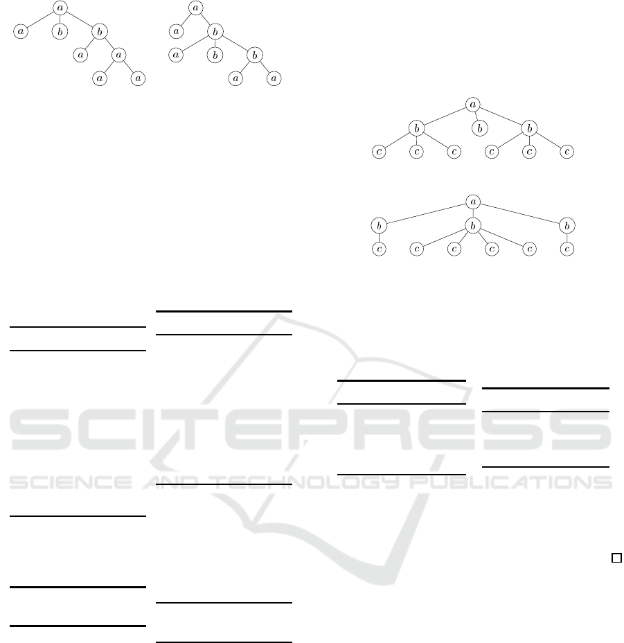
Example 1. Let C

and C

be caterpillars illustrated

in Figure 1.

Then, we obtain the histograms H

LCA

)

and H

LCA

) illustrated in Table 1. Note

LCA Histogram Distance for Rooted Labeled Caterpillars

309

Figure 1: The caterpillars C

and C

in Example 1.

that, since |C

| = |C

| = 8, it holds that

∑

p∈P (C

)

f(p,C

) =

= 28 for i = 1, 2. Also,

the bold faces illustrate the LCA pivots occurring in

either H

LCA

) or H

LCA

) and its frequency, or

the frequencies of the LCA pivot if they are different

in H

LCA

) and H

LCA

Table 1: The histograms H

LCA

) and H

LCA

) H

LCA

)

LCA pivots freq.

(a0 : a1⊔ b1) 2

(a0 : a1⊔ a2) 2

(a0 : a1⊔ a3) 2

(a0 : b1⊔ b1) 1

(a0 : b1⊔ a2) 2

(a0 : b1⊔ a3) 2

(a0 : a0⊔ a1) 1

(a0 : a0⊔ b1) 2

(a0 : a0⊔ a2) 2

(a0 : a0⊔ a3) 2

(b1 : a2⊔ a2) 1

(b1 : a2⊔ a3) 2

(b1 : b1⊔ a2) 2

(b1 : b1⊔ a3) 2

(a2 : a3⊔ a3) 1

(a2 : a2⊔ a3) 2

LCA pivots freq.

(a0 : a1⊔ b1) 1

(a0 : a1⊔ a2) 1

(a0 : a1⊔ b2) 2

(a0 : a1⊔ a3) 2

(a0 : a0⊔ a1) 1

(a0 : a0⊔ b1) 1

(a0 : a0⊔ a2) 1

(a0 : a0⊔ b2) 2

(a0 : a0⊔ a3) 2

(b1 : a2⊔ b2) 2

(b1 : a2⊔ a3) 2

(b1 : b2⊔ b2) 1

(b1 : b2⊔ a3) 2

(b1 : b1⊔ a2) 1

(b1 : b1⊔ b2) 2

(b1 : b1⊔ a3) 2

(b2 : a3⊔ a3) 1

(b2 : b2⊔ a3) 2

Hence, it holds that:

LCA

)

∑

p∈P (C

)∪P (C

)

| f(p,C

) − f(p,C

∑

p∈P (C

)\P (C

)

f(p,C

) +

∑

p∈P(C

)\P (C

)

f(p,C

)

∑

p∈P (C

)∩P (C

)

| f(p,C

) − f(p,C

= 9+ 14+ 5 = 28.

Whereas the LCA histogram distance seems to be

a metric, for example, Theorem 3.2 in (Tatikonda and

Parthasarathy, 2010), we show that it is not a metric

for trees as follows.

Theorem 3. There exist trees T

and T

such that

LCA

) = H

LCA

) but T

6= T

. Hence, the LCA

histogram distance is not a metric for trees in general.

Proof. Consider the trees T

and T

in Figure 2.

Figure 2: Trees T

and T

Then, we obtain the histogram H

LCA

)(=

LCA

)) illustrated in Table 2.

Table 2: The histogram H

LCA

)(= H

LCA

)).

LCA pivots freq.

(a0 : c2⊔ c2) 9

(a0 : b1⊔ c2) 12

(a0 : b1⊔ b1) 3

(a0 : a0⊔ b1) 3

LCA pivots freq.

(a0 : a0 ⊔ c2) 6

(b1 : c2⊔ c2) 6

(b1 : c2⊔ b1) 6

Here, since |T

| = |T

| = 10, it holds that

∑

p∈P (T

)

f(p,T

) =

= 45 for i = 1,2. Furthermore,

since the labels are not essential, this statement also

holds for unlabeled trees.

On the other hand, note that neither T

nor T

Figure 2 is a caterpillar. In the remainder of this sec-

tion, we discuss the LCA histogram distance between

caterpillars.

For caterpillars, the following lemma is obvious.

Lemma 1. Let p(v,w) = (l

: l

⊔ l

) ∈ P (C)

an LCA pivot in C. Then, the following statements

hold.

1. It holds that v⊔ w ∈ bb(C).

2. If v,w ∈ lv(C), then it holds that d

min{d

} − 1. Also it holds that v⊔w = par(v)

if d

< d

, v⊔ w = par(w) if d

< d

and v ⊔ w =

par(v) = par(w) if d

= d

3. If v,w ∈ bb(C), then it holds that d

min{d

}. Also it holds that v⊔w = v if d

< d

and v⊔ w = w if d

< d

KDIR 2018 - 10th International Conference on Knowledge Discovery and Information Retrieval

310

4. Suppose that v ∈ lv(C) and w ∈ bb(C). If d

< d

then it holds that d

= d

and v ⊔ w = w. Other-

wise, that is, d

≥ d

, it holds that d

= d

−1 and

v⊔ w = par(v).

Then, the following theorem holds.

Theorem 4. For caterpillars, the LCA histogram dis-

tance is a metric.

Proof. By the deﬁnition, it is sufﬁcient to show

that two caterpillars C

and C

are isomorphic iff

LCA

) = 0. In other words, it is sufﬁcient

to show that we can transform a caterpillar C from

LCA

By Lemma 1.1, we can uniquely determine bb(C)

from P (C) because of l

and d

in p(v, w). Since

lv(C) = C \ bb(C), we can determine lv(C). Then, by

Lemma 1.2, we can determine the set of leaves with

depth i for every i (1 ≤ i ≤ d(C)).

For λ

= |lv(C

)| and n

= |C

| (i = 1,2), it holds

that 0 ≤ δ

) ≤ λ

+ λ

, 0 ≤ δ

) ≤

+ n

and 0 ≤ δ

LCA

) ≤ (n

− 1)+ n

−

1))/2. Then, consider the extreme cases in Section 1.

Example 2. Let C

and C

be paths with length n.

Suppose that every vertex in C

is labeled by a and

that in C

by b. Then, it holds that τ

TAI

) = n,

) = 1, δ

) = 2n and δ

LCA

) =

2n(n − 1). Note that δ

), δ

) and

LCA

) are their maximum values.

Suppose that every vertex in C

and every non-

leaf vertex in C

is labeled by a and the leaf of C

is labeled by b. Then, it holds that τ

TAI

) = 1,

) = 1, δ

) = 2n and δ

LCA

) =

2(n − 1). Note that δ

) and δ

) are

their maximum values but δ

LCA

) is not.

In particular, δ

) cannot distinguish the dif-

ference of labels between two paths C

and C

Furthermore, the following theorem holds.

Theorem 5. There exist caterpillars C

and C

satis-

fying the following statements.

1. τ

TAI

) = δ

) = 1 but δ

) and

LCA

) are their maximum values.

2. δ

) and δ

) are their maximum

values but τ

TAI

) and δ

LCA

) are not.

Proof. 1. Let C

and C

be stars, that is, |bb(C

)| =

|bb(C

)| = 1, such that r(C

) = r

, r(C

) = r

, l(r

) 6=

l(r

), ch(r

) = ch(r

) and |ch(r

)| = |ch(r

)| = n−1.

Then, it is obvious that τ

TAI

) = δ

) =

1 and δ

) = 2(n − 1). Also, since P (C

) ∩

P (C

) =

0, it holds that δ

LCA

) = 2n(n− 1).

2. Let C

and C

be caterpillars obtained by con-

necting λ leaves to the leaves of paths with length h,

where every vertex in C

and in a path in C

is la-

beled by a and every leaf in C

by b. Then, |C

| =

| = h + λ = n. It is obvious that δ

) = 2λ

and δ

) = 2(λ + h) = 2n, so they are the

maximum values. On the other hand, it holds that

TAI

) = λ and δ

LCA

) = 2λ(n−1), where

their maximum values are 2n− 1 and 2n(n− 1).

By selecting every pair of vertices in two cater-

pillars, we can compute δ

LCA

) in O(n

) time,

because H

LCA

Note that the inequality that δ

< δ

LCA

tends

to hold by the values of δ

, δ

and δ

LCA

. Then, we

normalize δ

, δ

and δ

LCA

by dividing their maxi-

mum values when comparing distances. We denote

the normalized distances of δ

, δ

and δ

LCA

by δ

∗

and δ

∗

LCA

, respectively. Then, the following ex-

ample shows that the inequality that δ

∗

< δ

∗

< δ

∗

LCA

does not always hold.

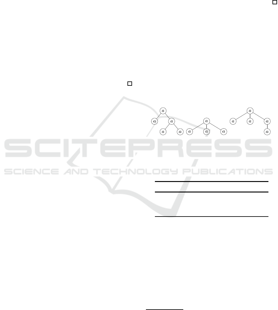
Example 3. Consider caterpillars C

, C

and C

Figure 3.

Figure 3: Caterpillars C

, C

and C

in Example 3.

Then, we obtain δ

), δ

LCA

), δ

∗

), δ

∗

) and δ

∗

LCA

)

for (i, j) = (1, 2),(1,3), (2,3) as follows.

(i, j) δ

LCA

∗

LCA

(1,2) 4 3 10 2/3 1/3 5/8

(1,3) 2 4 6 1/3 2/5 3/10

(2,3) 2 3 4 1/3 1/3 1/4

Hence, the following statements hold:

∗

) < δ

∗

LCA

) < δ

∗

LCA

) < δ

∗

) < δ

∗

LCA

) < δ

∗

) = δ

∗

4 EXPERIMENTAL RESULTS

Table 3 illustrates the number (#cat) of caterpillars in

the datasets in N-glycans and all of the glycans from

KEGG

, CSLOGS

and dblp

datasets, whose num-

ber of data is denoted by #data.

Kyoto Encyclopedia of Genes and Genomes,

http://www.kegg.jp/

http://www.cs.rpi.edu/˜zaki/www-new/pmwiki.php

/Software/Software

http://dblp.uni-trier.de/

LCA Histogram Distance for Rooted Labeled Caterpillars

311

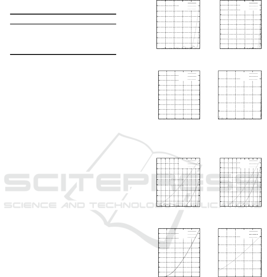
Table 3: The number of caterpillars in N-glycans and all-

glycans from KEGG, CSLOGS and dblp datasets.

dataset #cat #data %

N-glycans 514 2,142 23.996

all-glycans 8,005 10,704 74.785

CSLOGS 41,592 59,691 69.679

dblp 5,154,295 5,154,530 99.995

We deal with caterpillars for N-glycans, all-

glycans, CSLOGS and the selected 50,000 caterpil-

lars in dblp (we refer to dblp

−

). Table 4 illustrates

the information of such caterpillars. Here, ([a,b];c)

means that a, b and c are the minimum, the maximum

and the average number.

In the remainder of this section, we compare the

LCA histogram distance with the path histogram dis-

tance and the complete subtree histogram distance for

caterpillars.

Table 5 illustrates the running time of computing

∗

, δ

∗

and δ

∗

LCA

for N-glycans, all-glycans, CSLOGS

and dblp

−

Table 5 shows that, whereas we compute δ

∗

and

∗

in linear time and δ

∗

LCA

in quadratic time in theo-

retical, the running time of computing δ

∗

LCA

is within

twice for N-glycans and all-glycans, within thrice for

CSLOGS and about seven times for dblp

−

, respec-

tively, of computing δ

∗

in experimental. The rea-

son why the running time of computing δ

∗

LCA

is not

so large is that the number of |H

LCA

| is not so large

except dblp

−

; For dblp

−

, |H

LCA

| is larger than others

because the number of leaves is large but the height is

small in Table 4.

Figure 4 illustrates the distributions of δ

∗

, δ

∗

and

∗

LCA

for N-glycans, all-glycans, CSLOGS and dblp

−

Figure 4 shows that almost of the distributions

concentrate near to 1, in particular, CSLOGS and

dblp

−

. On the other hand, for dblp

−

, the distributions

appear near to 0. For N-glycans and all-glycans, δ

∗

larger than δ

∗

and δ

∗

is larger than δ

∗

LCA

Figure 5 illustrates the detailed distributions of δ

∗

and δ

∗

LCA

for N-glycans, all-glycans, CSLOGS

and dblp

−

, where the scopes of the distances of N-

glycans, all-glycans, CSLOGS and dblp

−

are [0.8,1],

[0.9,1], [0.995,1] and [0.99.1], respectively.

Note that, for dblp

−

, since the maximum value of

∗

is 0.992308 and the frequency is low, the distribu-

tion is just of δ

∗

and δ

∗

LCA

. Figure 5 shows that, near

to 1 and for N-glycans, all-glycans and CSLOGS, the

inequality of δ

∗

< δ

∗

< δ

∗

LCA

holds.

Figure 6 illustrates the scatter charts of δ

∗

, δ

∗

and

∗

LCA

for N-glycans and all-glycans and Figure 7 illus-

trates those for CSLOGS and dblp

−

, and their cor-

relation coefﬁcients (cc). Here, the representation of

0 0.2 0.4 0.6 0.8 1

percentage(%)

distance

LCA

path

100

0 0.2 0.4 0.6 0.8 1

percentage(%)

distance

LCA

path

N-glycans all-glycans

100

0 0.2 0.4 0.6 0.8 1

percentage(%)

distance

LCA

path

0 0.2 0.4 0.6 0.8 1

percentage(%)

distance

LCA

path

CSLOGS dblp

−

Figure 4: The distributions of δ

∗

, δ

∗

and δ

∗

LCA

for N-

glycans, all-glycans, CSLOGS and dblp

−

0.8 0.82 0.84 0.86 0.88 0.9 0.92 0.94 0.96 0.98 1

percentage(%)

distance

LCA

path

100

0.9 0.91 0.92 0.93 0.94 0.95 0.96 0.97 0.98 0.99 1

percentage(%)

distance

LCA

path

N-glycans all-glycans

100

0.995 0.996 0.997 0.998 0.999 1

percentage(%)

distance

LCA

path

0.99 0.992 0.994 0.996 0.998 1

percentage(%)

distance

LCA

path

CSLOGS dblp

−

Figure 5: The detailed distributions of δ

∗

, δ

∗

and δ

∗

LCA

for

N-glycans, all-glycans, CSLOGS and dblp

−

∗

/δ

∗

means that the number of pairs of caterpillars

with δ

∗

is pointed at the x-axis and that with δ

∗

pointed at the y-axis.

Figures 6 and 7 show that, the scatter charts for N-

glycans and all-glycans in Figure 6 are more sparse

than those for CSLOGS and dblp

−

in Figure 7, be-

cause the number of caterpillars in N-glycans and

all-glycans is much smaller than that in CSLOGS

KDIR 2018 - 10th International Conference on Knowledge Discovery and Information Retrieval

312

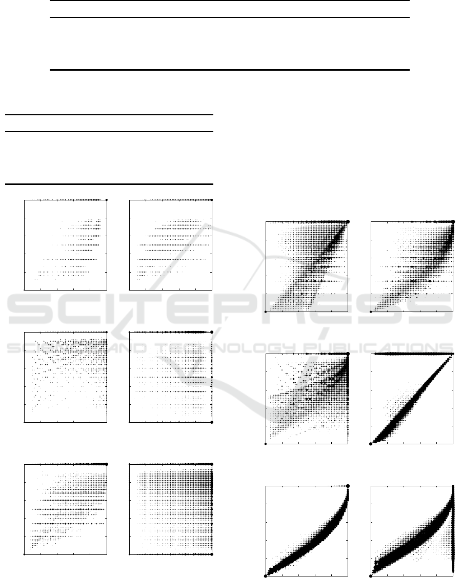
Table 4: The information of caterpillars in N-glycans, all-glycans, CSLOGS and dblp

−

dataset #vertices degree height #leaves #labels

N-glycans ([6,15];6.40) ([1,3];1.84) ([1,9];4.22) ([1,7];2.18) ([2,8];4.50)

all-glycans ([1,24];4.74) ([0,5];1.49) ([0,15];3.02) ([1,14];1.72) ([1,9];2.84)

CSLOGS ([2,404];5.84) ([1,403];3.05) ([1,70];2.20) ([1,403];3.64) ([2,168];5.18)

dblp

−

([7,244];11.96) ([6,243];10.94) ([1,3];1.02) ([6,243];10.94) ([7,13];9.86)

Table 5: The running time of computing δ

∗

, δ

∗

and δ

∗

LCA

(msec.).

dataset δ

∗

LCA

N-glycans 142 239 419

all-glycans 34,113 40,364 73,219

CSLOGS 1,017,730 1,361,343 3,439,560

dblp

−

1,980,062 3,534,120 24,633,812

0.2

0.4

0.6

0.8

0 0.2 0.4 0.6 0.8 1

path

0.2

0.4

0.6

0.8

0 0.2 0.4 0.6 0.8 1

path

LCA

N-glycans, δ

∗

/δ

∗

N-glycans, δ

∗

/δ

∗

LCA

cc = 0.402189 cc = 0.804891

0.2

0.4

0.6

0.8

0 0.2 0.4 0.6 0.8 1

LCA

0.2

0.4

0.6

0.8

0 0.2 0.4 0.6 0.8 1

path

N-glycans, δ

/δ

LCA

all-glycans, δ

∗

/δ

∗

cc = 0.356957 cc = 0.281586

0.2

0.4

0.6

0.8

0 0.2 0.4 0.6 0.8 1

path

LCA

0.2

0.4

0.6

0.8

0 0.2 0.4 0.6 0.8 1

LCA

all-glycans, δ

∗

/δ

∗

LCA

all-glycans, δ

∗

/δ

∗

LCA

cc = 0.571927 cc = 0.413714

Figure 6: The scatter charts of δ

∗

, δ

∗

and δ

∗

LCA

for N-

glycans and all-glycans.

and dblp

−

. Also for all datasets, the scatter chart

for δ

∗

/δ

∗

LCA

spreads more widely than those for

∗

/δ

∗

LCA

and δ

∗

/δ

∗

For Figure 6, the scatter charts for N-glycans have

the values on the line that y = 1 and, in particular, the

scatter charts of δ

∗

/δ

∗

LCA

also have the values on the

line that x = 1. On the other hand, the scatter charts

for all-glycans have the values on the line that y = 1,

those of δ

∗

/δ

∗

and δ

∗

/δ

∗

LCA

the vales on the lines

that x = 1 and y = 0.

0.2

0.4

0.6

0.8

0 0.2 0.4 0.6 0.8 1

path

0.2

0.4

0.6

0.8

0 0.2 0.4 0.6 0.8 1

path

LCA

CSLOGS, δ

∗

/δ

∗

CSLOGS, δ

∗

/δ

∗

LCA

cc = 0.735274 cc = 0.841885

0.2

0.4

0.6

0.8

0 0.2 0.4 0.6 0.8 1

LCA

0.2

0.4

0.6

0.8

0 0.2 0.4 0.6 0.8 1

path

CSLOGS, δ

∗

/δ

∗

LCA

dblp

−

, δ

∗

/δ

∗

cc = 0.645293 cc = 0.568405

0.2

0.4

0.6

0.8

0 0.2 0.4 0.6 0.8 1

path

LCA

0.2

0.4

0.6

0.8

0 0.2 0.4 0.6 0.8 1

LCA

dblp

−

, δ

/δ

LCA

dblp

−

, δ

∗

/δ

∗

LCA

cc = 0.980705 cc = 0.644874

Figure 7: The scatter charts δ

∗

, δ

∗

and δ

∗

LCA

for CSLOGS

and dblp

−

and their correlation coefﬁcients (cc).

LCA Histogram Distance for Rooted Labeled Caterpillars

313

For Figure 7, the scatter charts for CSLOGS have

the values on the line that y = 1 and those of δ

∗

/δ

∗

LCA

have the values on the line that x = 1. On the other

hand, the scatter charts of δ

∗

/δ

∗

for dblp

−

have the

values on the line that y = 1 and those of δ

∗

/δ

∗

LCA

have the values on the line that x = 1. In particular,

the scatter charts for dblp

−

constitutes at most two

clusters, where one lies on the axis.

For correlation coefﬁcients, which we denote by

cc(δ

∗

/δ

∗

), the value of cc(δ

∗

/δ

∗

LCA

) is highest for all

the data. On the other hand, it holds that

cc(δ

∗

/δ

∗

LCA

) < cc(δ

∗

/δ

∗

) < cc(δ

∗

/δ

∗

LCA

)

for N-glycans and CSLOGS, whereas it holds that

cc(δ

∗

/δ

∗

) < cc(δ

∗

/δ

∗

LCA

) < cc(δ

∗

/δ

∗

LCA

)

for all-glycans and dblp

−

. For the values of corre-

lation coefﬁcients, almost of the distances are related

for CSLOGS and dblp

−

, because cc(δ

/δ

) is greater

than 0.6, just δ

∗

LCA

is related with δ

∗

for N-glycans,

and no distances are related for all-glycans. In par-

ticular, cc(δ

∗

LCA

) is greater than 0.8 for N-glycans,

CSLOGS and dblp

−

5 CONCLUSION

In this paper, we have introduced an LCA histogram

distance δ

LCA

between trees and shown that it is not

a metric for trees but is a metric for caterpillars. Fur-

thermore, we have given experimental results of com-

puting δ

LCA

for caterpillars, by comparing the path

histogram distance δ

and the complete subtree his-

togram distance δ

(or their normalized distances

∗

LCA

, δ

∗

and δ

∗

It is a future work to design the algorithm to com-

pute δ

LCA

more efﬁciently, without constructing LCA

histograms explicitly, for example. It is also a future

work to analyze the relationship between δ

LCA

, δ

and

(or δ

∗

LCA

, δ

∗

and δ

∗

) in more detail in experimen-

tal, in particular, as stated in Section 4, to analyze why

the correlation coefﬁcients of δ

∗

and δ

∗

LCA

have been

high, and that in theoretical.

Furthermore, it is a future work to give experimen-

tal results for other data of caterpillars. Finally, it is

an important future work to analyze the relationship

between δ

LCA

and τ

TAI

(Muraka et al., 2018).

ACKNOWLEDGEMENTS

This work is partially supported by Grant-in-Aid

for Scientiﬁc Research 17H00762, 16H02870 and

16H01743 from the Ministry of Education, Culture,

Sports, Science and Technology, Japan.

REFERENCES

Akutsu, T., Fukagawa, D., Halld´orsson, M. M., Takasu, A.,

and Tanaka, K. (2013). Approximation and parame-

terized algorithms for common subtrees and edit dis-

tance between unordered trees. Theoret. Comput. Sci.,

470:10–22.

Aratsu, T., Hirata, K., and Kuboyama, T. (2009). Sibling

distance for rooted labeled trees. In JSAI PAKDD’08

Post-Workshop Proc. (LNAI 5433), pages 99–110.

Gallian, J. A. (2007). A dynamic survey of graph labeling.

Electorn. J. Combin., 14:DS6.

Kailing, K., Kriegel, H.-P., Sch¨onaur, S., and Seidl, T.

(2004). Efﬁcient similarity search for hierarchical data

in large databases. In Proc. EDBT’04, pages 676–693.

Kawaguchi, T., Yoshino, T., and Hirata, K. (2018a). Path

histogram distance and complete subtree histogram

distance for rooted labeled caterpillars. (submitted).

Kawaguchi, T., Yoshino, T., and Hirata, K. (2018b). Path

histogram distance for rooted labeled caterpillars. In

Proc. ACIIDS’18 (LNAI 10751), pages 276–286.

Li, F., Wang, H., Li, J., and Gao, H. (2013). A survey on

tree edit distance lower bound estimation techniques

for similarity join on XML data. SIGMOD Record,

43:29–39.

Muraka, K., Yoshino, T., and Hirata, K. (2018). Computing

edit distance between rooted labeled caterpillars. In

Proc. FedCSIS’18 (to appear).

Tai, K.-C. (1979). The tree-to-tree correction problem. J.

ACM, 26:422–433.

Tatikonda, S. and Parthasarathy, S. (2010). Hashing tree-

structured data: Methods and applications. In Proc.

ICDM’10, pages 429–440.

Zhang, K. and Jiang, T. (1994). Some MAX SNP-hard re-

sults concerning unordered labeled trees. Inform. Pro-

cess. Lett., 49:249–254.

KDIR 2018 - 10th International Conference on Knowledge Discovery and Information Retrieval

314