Safe Driving Mechanism: Detection, Recognition and Avoidance of

Road Obstacles

Andrea Ortalda

1,3

, Abdallah Moujahid

2,3

, Manolo Dulva Hina

Assia Soukane

and Amar Ramdane-Cherif

Politecnico di Torino, 24 Corso Duca degli Abruzzi,10129 Turin, Italy

Université Internationale de Casablanca, Casablanca, Morocco

ECE Paris School of Engineering, 37 quai de Grenelle, 75015 Paris, France

Université de Versailles St-Quentin-en-Yvelines, 10-12 avenue de l’Europe, 78140 Velizy, France

Keywords: Ontology, Formal Specification, Machine Learning, Safe Driving, Smart Vehicle, Cognitive Informatics.

Abstract: In an intelligent vehicle (autonomous or semi-autonomous), detection and recognition of road obstacle is very

important for it is the failure to recognize an obstacle on time which is the primary reason for road vehicular

accidents that very often leads to human fatalities. In the intelligent vehicle of the future, safe driving is a

primary consideration. This is accomplished by integrating features what will assist drivers in times of needs,

one of which is avoidance of obstacle. In this paper, our knowledge engineering is focused on the detection,

classification and avoidance of road obstacles. Ontology and formal specifications are used to describe such

mechanism. Different supervised learning algorithms are used to recognize and classify obstacles. The

avoidance of obstacles is implemented using reinforcement learning. This work is a contribution to the

ongoing research in safe driving, and a specific application of the use of machine learning to prevent road

accidents.

1 INTRODUCTION

The statistics on global traffic accidents

(World_Health_Organization 2017) are disturbing:

 Every year, about 1.24 million people die each

year in road traffic accidents;

 Road traffic injury is the leading cause of death

on young people, aged 15–29 years;

 Half of those dying on the world’s roads are

“vulnerable road users”, namely the

pedestrians, cyclists and motorcyclists;

 If no remedy is employed, road traffic

accidents are predicted to result in the deaths of

around 1.9 million people annually by 2020.

Here lies the importance of researches on

intelligent transportation intended to detect,

recognize and avoid road obstacles, such as ours. An

intelligent transportation (Kannan et al. 2010)

(Fernandez et al. 2016) denotes advanced application

embodying intelligence to provide innovative

services related to road obstacles, enabling various

users to be better informed and makes safer, more

coordinated, and smarter decisions.

Our vision of an innovative vehicle (Hina et al.

2017) is shown in Figure 1. Within this vehicle is an

intelligent architecture with three main components:

(1) Embedded System, (2) Intelligent System, and (3)

Network and Real-time System.

Figure 1: Smart services for an intelligent vehicle.

Ortalda, A., Moujahid, A., Hina, M., Soukane, A. and Ramdane-Cherif, A.

Safe Driving Mechanism: Detection, Recognition and Avoidance of Road Obstacles.

DOI: 10.5220/0006935400960107

In Proceedings of the 10th International Joint Conference on Knowledge Discovery, Knowledge Engineering and Knowledge Management (IC3K 2018) - Volume 2: KEOD, pages 96-107

ISBN: 978-989-758-330-8

The intelligent system component, for its part, has

a built-in intelligence that enables the vehicle to

detect, classify and avoid an obstacle. Embedded

Machine learning (Ithape 2017, Saxena 2017)

intelligence makes it appropriate to decide on behalf

of the driver and other passengers. In this paper, we

explain machine learning and types of machine

learning in details. We intend to use machine learning

in the detection, classification and avoidance of

obstacles. To realize this, we developed a driving

setting in which the driving environment is described.

In such environment, we distinguished the road

objects, the near objects and the obstacles. We then

make use of supervise learning to identify and

classify these obstacles. The work is completed by

designing reinforcement learning mechanism to

avoid a generic obstacle. The case is applicable to all

other types of obstacles.

2 RELATED WORKS

Many researches have been made on obstacle

detection, classification and avoidance as this type of

system helps insuring road safety and therefore has

become one of the key enablers in Advanced Driver

Assistance System (ADAS). For example, the Euro

New Car Assessment Program requires providing

vehicles with a Front Collision Warning function

(Pyo et al. 2016). Several carmakers started

implementing obstacle detection and avoidance based

systems such as Front Assist, Crash avoidance and

Automatic Emergency Braking (AEB) in their middle

and high range cars (Coelingh et al. 2010,

ResearchNews 2013). Image processing techniques

and computer vision models are extensively used in

obstacle detection and classification researches

(Bevilacqua and Vaccari 2007, Zeng et al. 2008)

(Wolcott and Eustice 2016). This is justified by the

use of different types of cameras such as stereo and

monocular ones, which are less expensive than high-

density laser scanners like LiDAR (Levi et al. 2015).

Other research works, such as (Linzmeier et al. 2005,

Bertozzi et al. 2008, García et al. 2013, Shinzato et al.

2014, Wang et al. 2014) use combined information

obtained from several lasers and imaging sensors to

detect road obstacles namely vehicles and

pedestrians. The main reason being the

complementarity between these different sensors and

the fact that the imaging sensors do not provide

enough information on the distance between the

vehicle and the obstacles of the road, which is

essential for obstacle avoidance systems.

In (Bazilinskyy et al. 2018), the authors proposed

a system based on a deep network for road scene

visualization (Figure 2). The system generates a

bird’s eye map showing the surrounding vehicles that

are visible to the dashboard camera. To train the

model, authors used a video game called GTAV to

generate a massive dataset of more than one million

images. Each image has two variants, one

corresponding to vehicle dashboard view and the

second to bird’s eye view. Other information like

yaw, location and distance are also collected. Authors

claims the usefulness of the system to help the driver

in making a better decision being more aware of the

driving environment.

Figure 2: Input and output of Bazilinskyy, P. et al. system.

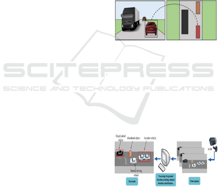
The authors in (Lan et al. 2016) worked on a real-

time approach to detect and recognize road obstacles.

A special focus has been made on three types of

obstacles, namely abandoned objects, illegally parked

vehicles and accident vehicles (Figure 3). The system

follows three main consequent steps. It starts by

removing the objects outside the road using a Flushed

Region of Interest (FROI) algorithm. It then uses a

Histogram Orientation Gradient (HOG) descriptor to

detect road obstacles based on the speed of tracked

objects and finally applying a Support Vector

Machine (SVM) algorithm to classify the ROI and to

separate abandoned objects from vehicles (both

accident and illegally parked vehicles).

Figure 3: Overview of detection system.

The two types of vehicles are then distinguished

using a special algorithm for accident vehicles

identification. The authors contend that the proposed

system achieved a detection rate of 96%.

Safe Driving Mechanism: Detection, Recognition and Avoidance of Road Obstacles

Most of collision avoidance systems start by

detecting and classifying the obstacle that may cause

the collision before calculating the time to collision

(TTC) which indicates the remaining time two

consecutive vehicles are to collide. In the event of

TTC, the system reacts either by alerting or warning

the driver or even by acting on the vehicle causing

braking (Rummelhard et al. 2016). In 2011, Volvo

has commercialized its “Volvo S60” car with

"Collision Warning with Auto Brake and Cyclist and

Pedestrian Detection" feature to assist the driver in

case of a risk of collision with a vehicle, cyclist or

pedestrian (Coelingh, Eidehall et al. 2010). Other

auto manufacturers such as Ford, Honda, and Nissan

Mercedes-Benz have equipped their vehicles with

Collision Avoidance Systems (ResearchNews 2013).

The authors of (Shinzato, Wolf et al. 2014)

proposed an obstacle detection method that processes

a data from a LIDAR sensor combined with single

camera-generated images. The obstacles are then

classified using the LIDAR point’s height

information. In (Lee and Yeo 2016), the authors

proposed a system for real time Collision Warning

based on a Multi-Layer Perceptron Neural Network

(MLPNN). The input layer was composed of five

input neurons: the distance between preceding and

following vehicle, speed and acceleration of the

following vehicle, speed and deceleration of the

preceding vehicle. The final output used a threshold

discriminator of 0.5 to come out with a value of zero

or one indicating whether a rear-end collision

warning should be displayed.

In (Iqbal et al. 2015), the authors worked on a

Dynamic Bayesian Network (DBN) method to train a

model using information gathered by IMU sensor and

a camera. The system was designed to provide two

types of support: warning on nearby vehicles and

brake alert for potential collision with the calculation

of the speed and acceleration of the vehicle. The test

showed a convenient performance that can be

improved by adding other sensors like radar and

LIDAR. Most features here have to be integrated in

smart vehicle’s intelligent component.

3 THE DRIVING ENVIRONMENT

The driving environment is a set of all the elements

describing the driver, the vehicle and all entities,

animate or inanimate, present during the conduct of a

driving activity. In this section, we will analyse the

features that makes an object found within the

environment an obstacle.

3.1 Environment Representation

Here, we identify the elements that are present during

the conduct of a driving activity. We will describe

these elements in a mathematical notion. The sets of

elements present in the environment during a driving

activity are: (i) the road object collection (R); (ii) the

nearby object collection (C); and (iii) the obstacle

object collection (O)

Let R be the set of all the road objects present in

the environment E. Let C be the set of nearby road

objects and O the set of the obstacles. Then R is an

element of E, C is a subset of R, and O is a subset of

C. Mathematically,

R = {r

, r

, …, r

}, R ⊂ E (1)

C = {c

, c

, …, c

}, C ⊆ R (2)

O = {o

, o

, …, o

}, O ⊆ C (3)

Let

e be an environment object in our driving

simulation platform, programmed using Unity 3D

(Game_Engine 2016). Every

e related to the driving

environment has a tag

t, a notation used for

identification purposes. For all

e in E, if an element e

has a tag of “

RoadObject”, then such e (denoted e

) is

a road object

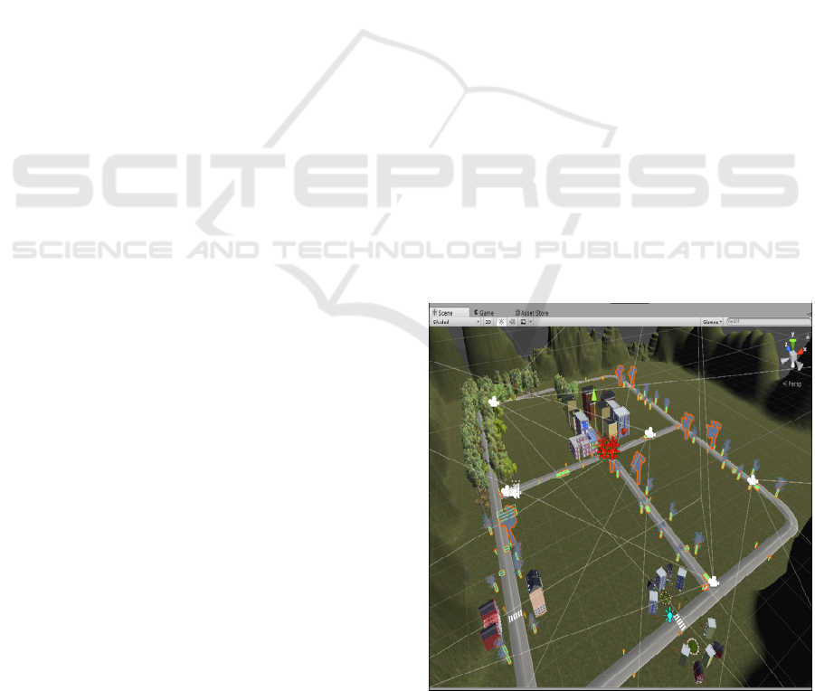
. Mathematically, ∀e ϵ E | ∃e

• t =

“RoadObject”  e

= r

∧ R ≠ ∅. Figure 4 shows the

specimen environment E and all the elements

r ϵ R

(all elements that are found on the road) are

highlighted.

Figure 4: The specimen environment E and the entire road

objects r’s therein (R ⊂ E).

KEOD 2018 - 10th International Conference on Knowledge Engineering and Ontology Development

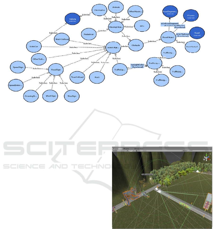
Figure 5: The ontological representation of road object collection R.

Figure 5 shows the ontological representation of

an element

r ∈ R. The subclasses describe the

different types of r and every subclass of Thing can

have one or more individuals. The arrows

“

hasSubclass” and “hasIndividual” show how this is

done in Protégé (Protégé 2016).

3.2 The Nearby Road Object Collection

The nearby road objects are those elements that are

within the vicinity of the referenced vehicle. See

Figure 6. They are parts of the road objects collection.

By vicinity, we mean an element is located within the

referenced radius (example: 50 meters) of a

referenced vehicle. Let

m be the radius of the

referenced sphere (as it is the case in Unity 3D), and

d as the distance between our referenced vehicle and

a road object. If the distance d of the road object is

less than m then such road object is considered a

nearby road object

c. Mathematically, ∀r ϵ R | ∃r

• d

< m  r

= c

∧ C ≠ ∅.

Figure 6 shows our specimen E with all elements

c ∈ C highlighted. Take note that a radius from the

referenced vehicle is shown. It is to be noted that this

one is just one of the possible

c to consider. Nearby

road objects may be in front, at the back, on the left

or on the right side of the referenced vehicles. Some

of the nearby road objects may be obstacles while

some may be not. Ontology creation is therefore

important because it allows us to have a good vision

of the closest road object that may be considered as

road obstacles.

Figure 7 shows all elements

c ∈ C. As shown, the

ontology is much smaller than the previous one, given

that we only consider objects that are present in the

specified radius of a sphere with our vehicle as the

point of reference, with radius =

Figure 6: The nearby road objects from the referenced

vehicle’s perspective.

3.3 The Obstacle Object Collection

The nearby road objects are obstacles if they are in

front of the vehicle (located in the same lane), the

distance between it and the referenced vehicle is near,

and the time to collision is near.

Let

v = the current speed of our referenced vehicle,

d = the distance between the vehicle and the road

object r, t = the time to collision, m = radius of the

Safe Driving Mechanism: Detection, Recognition and Avoidance of Road Obstacles

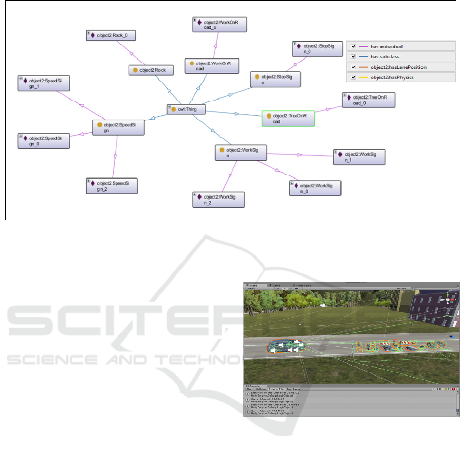
Figure 7: The ontological representation of nearby road object collection C.

sensor sphere, l = describes if the vehicle and the

object

r are on the same lane and p = the direction of

the vehicle. For a nearby object

∈ C located within

the vicinity of the referenced vehicle, and given that

the speed of the vehicle divided by the distance

between the vehicle and the nearby object is less than

the time to collision, and that both the vehicle and the

nearby object are on the same lane, then object

an obstacle. Mathematically, ∀

c ϵ C | ∃c

• d < m ∧ v/d

< t ∧ l = 1 ∧

d > 0  c

= o

∧ O ≠ ∅. Note that the

parameter

p is used in the computation of l.

Given that the simulation platform is in 3D

coordinate system, the orientation is necessary in

order to determine if vehicle

s and nearby object c are

on the same lane. Let

dcr be the distance from the

center of the road. Then:

 If

p = North ∨ p = South  dcr is taken on the

x plane, else  dcr is taken on the z plane.

Let dcr

be the distance the vehicular system to the

center of the road, and dcr

be the distance of nearby

object to the center of the road, then:

 l =1, if (dcr

> 0 ∧ dcr

> 0) ∨ (dcr

< 0 ∧ dcr

 l = -1, if (dcr

> 0 ∧ dcr

< 0) ∨ (dcr

< 0 ∧ dcr

> 0)

Figure 8 shows a sample road obstacle located in

the same lane as the vehicle. Here, the ontology

representation details are important. It is essential that

all conditions for qualifying an object as an obstacle

be verified.

Figure 8: A sample obstacle in the simulation platform.

Figure 9 shows the properties of every obstacle o

∈ O. Here, the ontology is presented in details for

obstacle roadwork

∈ O. The legend below shows

the obstacle characteristics, such as speed or size.

In this phase, the road obstacle is already detected.

The next phase should be the identification of the

obstacle. An obstacle may be another vehicle (static

or moving), a pedestrian, a roadwork sign, a traffic

light, etc. In general, when an obstacle is detected, the

referenced vehicle should stop or slow down and try

to avoid such obstacle. The manner to avoid is

different, depending on the type of the obstacle. For

example, we avoid pedestrian differently from a rock

stuck on the road. Machine learning (Mitchell 1997,

Louridas and Ebert 2016) would be used to identify

an obstacle.

KEOD 2018 - 10th International Conference on Knowledge Engineering and Ontology Development

100

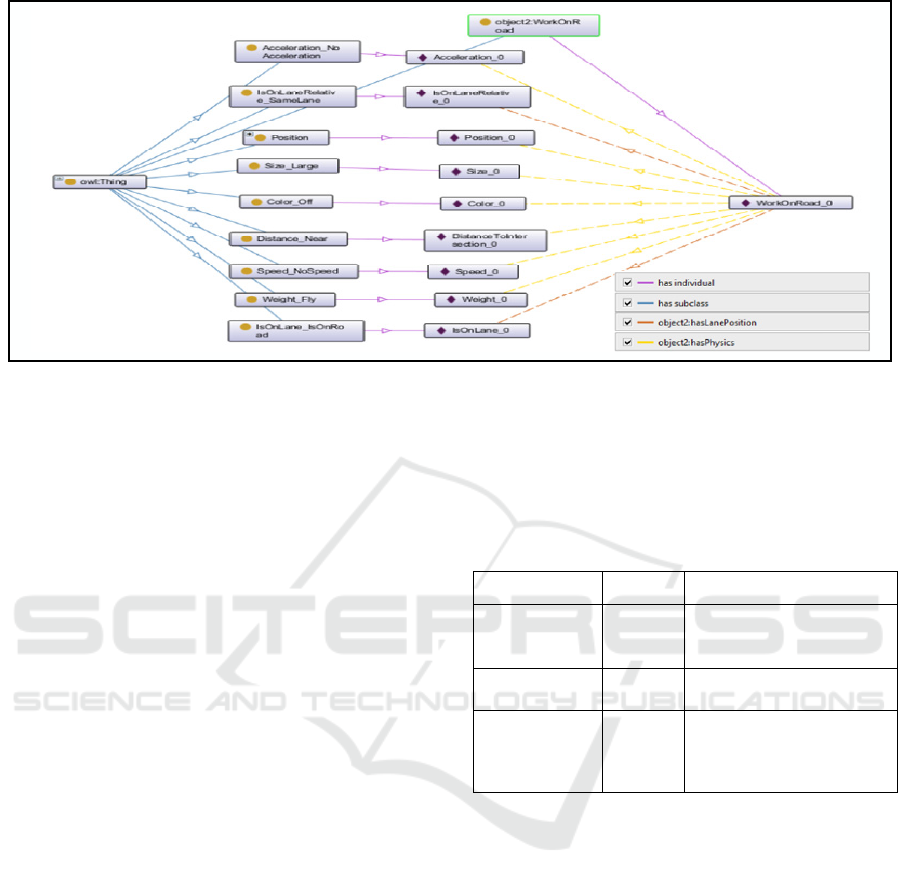
Figure 9: Ontological representation of a sample obstacle (work on the road).

4 MACHINE LEARNING FOR

OBSTACLE CLASSIFICATION

4.1 Basics of Machine Learning

Supervised learning and unsupervised learning are

the two main learning types in which we can divide

the machine-learning world (Tchankue et al. 2013),

while reinforcement learning and deep learning can

be seen as special application of supervised and

unsupervised learnings. Consider a normal

x-y

function, given a set of input x, we define y as the

corresponding output value for a relation f between

and y. The differences between machine learning

techniques may be explained using the basic notion

of mathematics given below:

 In supervised learning, x and y are known and

the goal is to learn a model that approximate

 In unsupervised learning, only

x is given and

the goal is to find

f between the set of x.

Supervised learning is used for model

approximation and prediction while unsupervised is

used for clustering and classification (Tchankue,

Wesson et al. 2013). Reinforcement learning is a

particular case of supervised learning; it differs from

the standard case not due to the absence of

y but in the

presence of delayed-reward

r that allows it to

determine f in order to get the right y. See Table 1.

Deep learning is a supervised or unsupervised

work based on learning data representation. It uses an

architecture based on multiple-layer structure for the

data (Lv et al. 2015), using it for feature extraction

and representation. Each successive layer uses as

input the previous layer output (Bengio 2009).

Table 1: Basic mathematical representation for machine

learning.

ML Method Relation Comments

Supervised

Learning

y = f(x)

x and y are known and the

goal is to learn a model

that approximates

Unsupervised

Learning

f(x)

x is given and the goal is to

find

f for a given set of x

Reinforcement

Learning

y = f(x);

r is a reward that allows

determination of f in

order to obtain the optimal

(Legend: red-colored symbol means unknown data and the

blue-colored symbol means known data)

4.2 Obstacle Classification using

Decision Tree

Decision tree learning uses a decision tree as a

predictive model. A decision tree is a flowchart-like

structure in which each internal node represent a

“test” on an attribute, each branch representing the

outcome of the test while each leaf representing a

class label for classification tree. A tree can be created

by splitting the training set into subset based on an

attribute value test and repeating the process until

each leaf of the tree contains a single class label or we

reach the desired maximum depth. There are multiple

criterion that can be used to divide a node into two

branch, such as the information gain, which consist of

finding the split that would give the biggest

Safe Driving Mechanism: Detection, Recognition and Avoidance of Road Obstacles

101

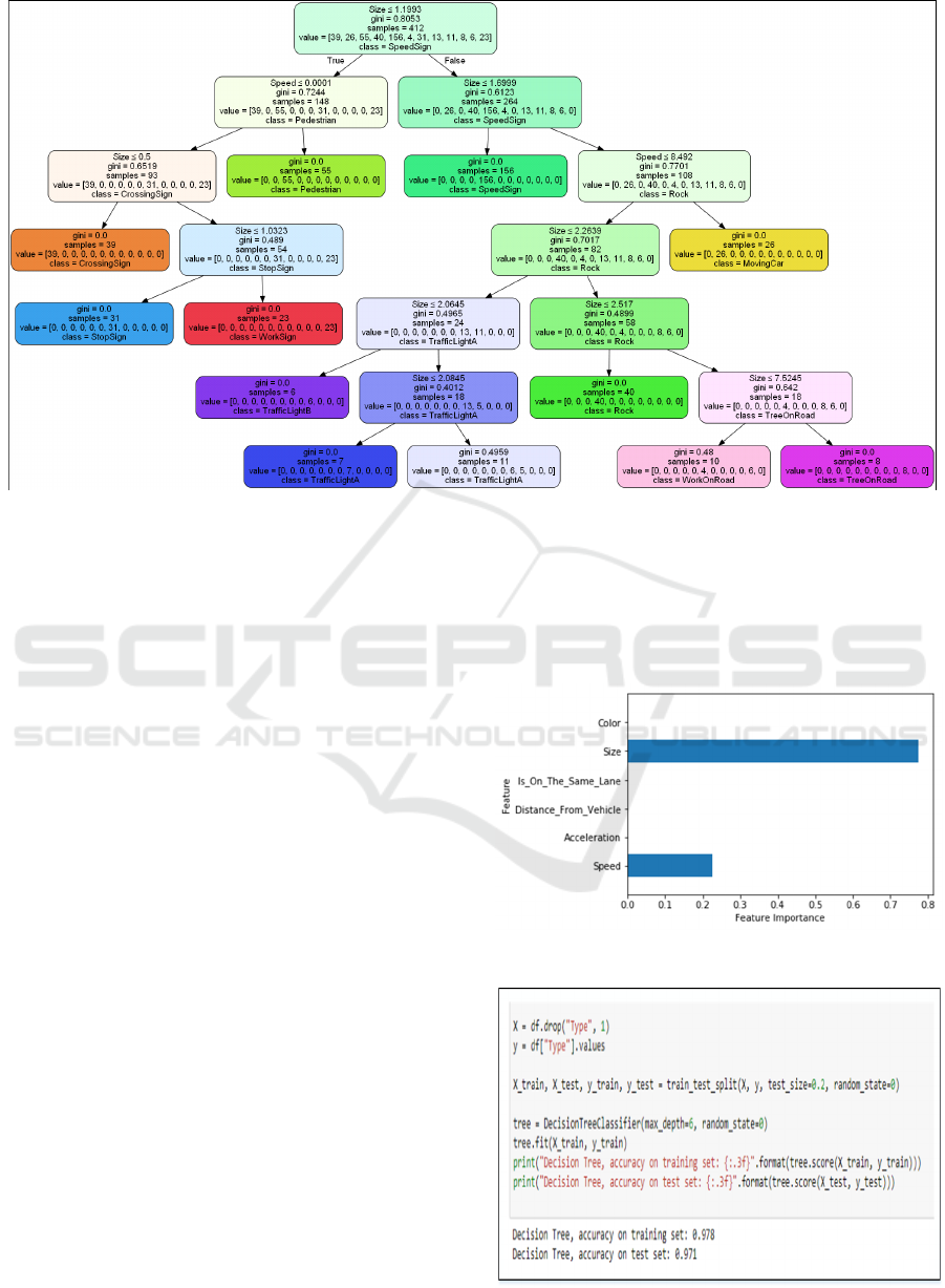
Figure 10: Obstacle classification using decision tree.

information gain, based on the entropy from the

information theory (Witten, Frank et al. 2011).

Figure 10 shows the decision tree created for the

object classification. Gini impurity is a measure of how

often a randomly chosen element from the set would

be incorrectly labeled if it were randomly labeled

according to the distribution of labels in the subset. The

value signifies various obstacles considered and value

= [crossingSign, movingCar, pedestrain, rock,

speedSign, workOnroad, stopSign, traffickLightA,

traffickLightB, treeOnRoad, staticCar, workSign].

Figure 11 shows the feature importance of the

decision tree. As shown, the feature that is most

important for the decision-tree classification

algorithm, as per simulation result, is the obstacle’s

size and speed; all others are not even considered.

Figure 12 shows the decision tree score in the

identification of an obstacle. It uses the data as 80%

for training, 20% for testing. Accordingly, it obtains

97.8% accuracy in identifying obstacles in the

training set and 97.1% in identifying the obstacles

within the test set. The results are satisfactory.

4.3 Obstacle Classification using

K-Nearest Neighbours (KNN)

The k-nearest neighbor algorithm is a simple

algorithm, which consists of selecting for an instance

of data the k-nearest other instances and assigning to

the first instance the most frequent label in the k

instance selected. The value of k is user defined. The

distance can be computed in different ways, such as the

Euclidian distance for continuous variables like ours.

The importance of each neighbor can be weighted;

often the weight used is inversely proportional to the

distance to give more importance to closer neighbor.

Figure 11: Obstacle classification using decision tree.

Figure 12: Decision tree score.

KEOD 2018 - 10th International Conference on Knowledge Engineering and Ontology Development

102

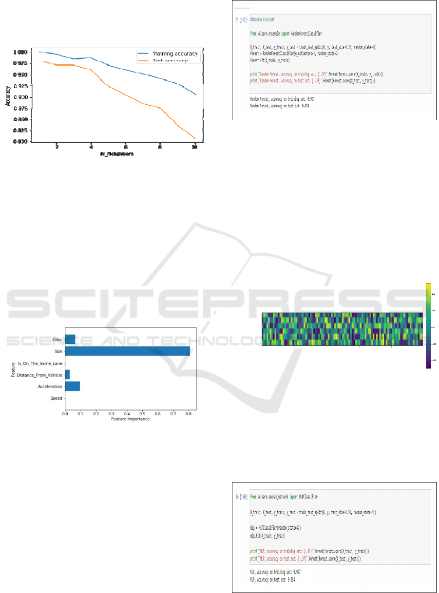
Figure 13 shows the KNN score for the data of

which 80% are used for training, and 20% for testing

for different values of k = [0, 10], k ∈ Ζ.

Figure 13: KNN prediction’s accuracy result for training

and testing with k = 0 to 10.

4.4 Obstacle Classification using

Random Forest

Random Forest is a supervised learning algorithm. It

creates a forest and makes it somehow random. The

“forest” it builds is an ensemble of decision trees,

most of the time trained with the “bagging” method.

The general idea of the bagging method is that a

combination of learning models increases the overall

result (Donges 2018). Figure 14 shows the feature

importance of the random forest.

Figure 14: Features involved in KNN obstacles

classification.

As shown, the feature that is most important for

the random-forest classification algorithm, as per

simulation result, is the obstacle’s size, acceleration,

color and the obstacle’s distance from the referenced

vehicle.

Figure 15 shows the random forest score in the

identification of an obstacle. It uses 70% of the data

for training, and 30% for testing. Accordingly, it

obtains 99.7% accuracy in identifying obstacles in the

training set and 99.4% in identifying the obstacles

within the test set. The results are better than the ones

obtained using decision-tree learning algorithm.

Figure 15: Random Forest score.

4.5 Obstacle Classification using

Multilayer Perceptron

A multilayer perceptron (MLP) is a feedforward

artificial neural network that generates a set of outputs

from a set of inputs. An MLP is characterized by

several layers of input nodes connected as a directed

graph between the input and output layers. MLP uses

back propagation for training the network. MLP is a

deep learning method (Technopedia 2018). Figure 16

shows the feature importance of the MLP classifier.

40 60 80

Colu mns in weight matrix

Speed

Acceleration

Distance from

Vehicle

Is On the Same Lane

Size

Col or

Input

Feature

Figure 16: MLP Classifier.

Figure 17 shows the MLP score in the

identification of an obstacle. It uses 70% of the data

for training, and 30% for testing. Accordingly, it

obtains 99.7% accuracy in identifying obstacles in the

training set and 99.4% in identifying the obstacles

within the test set. The results are the same as the ones

from random forest learning algorithm

Figure 17: MLP Score.

Safe Driving Mechanism: Detection, Recognition and Avoidance of Road Obstacles

103

6 OBSTACLE AVOIDANCE

After the obstacle detection, the system needs to

avoid the obstacle. This will be done using a

reinforcement learning application, building a

Markov decision process (MDP) (Sutton and Barto

2017). From a mathematical point of view,

reinforcement-learning problems are always

formalized as Markov decision process, which

provides the mathematical rules for decision making

problems, both for describing them and their

solutions. A MDP is composed by five elements, as

shown in Table 2:

Table 2: Basic elements of Markov decision process.

Variable Definition

State

S is the finite set of the possible states in

an environment

Action

A is the possible set of action available for

a state S.

Environment

T(S, A, S’); P(S

’

|A, S) where T represents

the environment model: It is a function

that produces the probability

P of being in

state

S’ taking action A in the state S.

Reward

R(S, A, S’) is the reward given by the

environment for passing from

S’ to S as a

consequence of A

Policy

π(S; A) is the policy of the state (i.e.

The solution of the problem) that takes as

input a state

S and gives the most

appropriate action

A to take.

The hypothesis here is the necessity to create a

Markov Decision Process (MDP) based on

S, A, and r

in order to get a policy

P able to avoid the obstacle in

our environment E.

 Action set

A = [Accelerate, Steer]

 Reward function r based on the vehicle lane

and collision with obstacles

 Possible state set

S (position of the vehicle in

the environment).

The action set is composed of two actions of

steering the vehicle, and accelerate (in a positive or

negative way), while the reward function is based on

the position of the vehicle with respect to the lane and

collision with obstacles:

 Positive reward if the vehicle stays on the road

and no collision occurs.

 Negative reward if the vehicle is no longer on

the road and a collision is detected.

Finally, the vehicle would at every time

t in

certain state s, represented by the position in the

environment.

6.1 The Reinforcement Learning (RL)

Scene

In order to test a working avoidance system, a new

scene was created. The scene, for simplicity purposes,

is composed of three main actors: a vehicle, an

obstacle and an intended destination. The idea is

simple: the vehicle must avoid (after detecting and

classifying) the obstacle. It must be able to get back

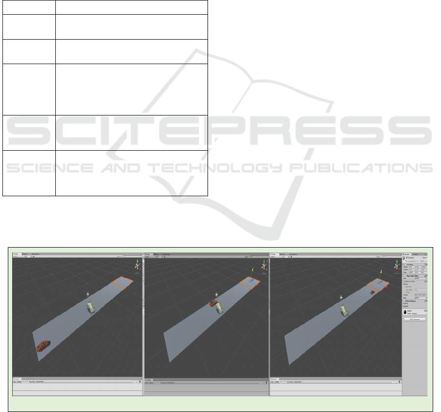
to its right lane afterwards. Figure 18 shows the

intended RL scene. The vehicle would be able to

detect the obstacle (Figure 18(a)), avoid it (Figure

18(b)) and get into its intended destination (Figure

18(c)). With various tests and trials, we are able to

achieve our goal at the end of the process.

(a) Before avoidance of an obstacle

(b) During the avoidance of an obstacle

Figure 18: Reinforcement Learning for Obstacle Avoidance: before, during and after the avoidance of obstacle.

KEOD 2018 - 10th International Conference on Knowledge Engineering and Ontology Development

104

6.1.1 Reward Function

The purpose of the reward function is for the vehicle

to avoid the obstacle and return to its intended

destination. Equations 4 and 5 show the reward

functions structure, where collision is a variable

whose value is 1 if the vehicle reaches its target

(intended destination) and 0 if collides with the

obstacle, isOnLane is a variable whose value is 1 as

long as the vehicle is on the road, otherwise its value

is 0. distanceToTarget and previousDistance are

variables updated every frame, representing the

current and the previous distance of the vehicle and

its intended destination.

=











+1=1

+0.1<

−0.05 >

−0.05<+1

−1 =0|| =0

(4)

=











+1=1

+0.05<

−0.05 >

−0.05 <+1

−1=0||=0

(5)

A key point in the reward function is the time

penalty factor: -0.05 for function 1 and -0.01 for

function 2. This small reward is added at every frame,

expressed with mathematical condition t

< t

i+1

. The

time penalty factor is used in the RL reward function

implementation, encouraging the agent to move and

reach the target. The best performances were

achieved with function 1, while function 2 showed

high values for reward function but with worst

performances.

Here, we present the three different training

results. For each result, a graph shows each of the two

most important statistics for the training phase. They

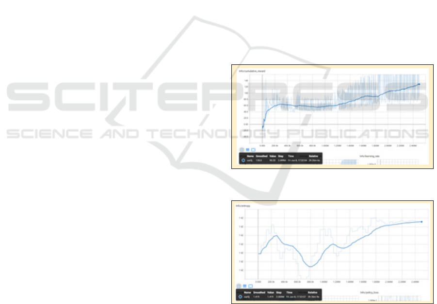
are described below:

1. Cumulative Reward: This is the mean cumulative

episode reward over all agents. It should increase

on a successful training session.

2. Entropy: It describes how random the decisions

of the model are. It should slowly decrease

during a successful training process.

All three trainings were made using same

parameters with only two changes: the reward

function used and the maximum step that fixes the

maximum number of steps for the training phase. The

next discussion focuses on the problems and strong

points in each training phase

6.1.2 Training 1: CarSimpleJ

Here, the first good performances were

accomplished using the following parameters, using

the 2 reward function:

default: trainer: ppo | batch_size: 4096

| beta: 1.0e-4 | buffer_size: 40960 |

epsilon: 0.1 | gamma: 0.99 |

hidden_units: 256 | lambd: 0.95 |

learning_rate: 1.0e-5 | max_steps: 2.5e6

| memory_size: 256 | normalize: false |

num_epoch: 3 | num_layers: 2 |

time_horizon: 64 | sequence_length: 64 |

summary_freq: 1000 | use_recurrent:

false

Figures 19 and 20 show the graphs for the

Cumulative Reward and Entropy of CarSimpleJ.

Here, the key point is that the reward is overall

increasing, but has lot of peaks, both high and low.

This is due to the Entropy that is not decreasing in the

right way. This leads to a behaviour that sometimes

gives us good results, and sometimes not, with the

vehicle either reaching its destination or colliding

with the obstacle.

Figure 19: Cumulative reward for carSimpleJ training.

Figure 20: Entropy for carSimpleJ training.

Compared with previous simulations, this

training, however, is the first one that gives us a

reward that overall was increasing, hence

accomplishing the task. The number of iterations,

however, is small (2.5 million). The results we

obtained here becomes the starting point for other

Safe Driving Mechanism: Detection, Recognition and Avoidance of Road Obstacles

105

simulations given that the parameters for the learning

phase were suitable for the application.

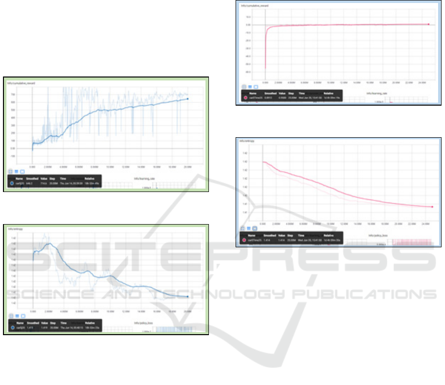
6.1.3 Training 2: CarSimpleJ20

Here, we made some changes on the maximum step

parameter, earlier fixed to 20 million, in order to see

if the reward and entropy would have followed the

correct behaviour. Figures 21 and 22 show the

behaviour of the parameters, highlighting the correct

trend, even with some low peaks for the reward.

Figure 21: Cumulative reward for carSimpleJ20 training.

Figure 22: Entropy for carSimpleJ20 training.

From a numerical point of view, the results were

very satisfying, but the problem was linked to the

vehicle’s behaviour. It was going too slow, taking

positive reward thanks to the fact it was getting closer

to the target destination. After the agent has avoided

the obstacle, it was not, however, able to return on the

correct lane. This overfitting behaviour was due to the

reward given when the target is approaching the

destination being too high relative to the value given

to the final goal to achieve. Note the difference of the

trend in the graph, Entropy for CarSimpleJ and

CarSimpleJ20 (Figure 20 and 22).

6.1.4 Training 3: CarSimpleJ25

The behaviour obtained in the previous simulations

has suggested that a change in the reward function is

necessary. Indeed, Equation 1 was adopted, changing

the value assigned for approaching the target and the

time penalty. In Figures 23 and 24, it is possible to

notice the immediate stabilization of the reward func-

tion, while the entropy is decreasing in the correct way.

Figure 23: Cumulative reward for carSimpleJ25 training.

Figure 24: Entropy for carSimpleJ25 training.

The behaviour is almost perfect, with the agent

able to avoid the obstacle and return in the correct

lane, reaching the intended destination. In this

simulation, the maximum step parameter was set to

25 million.

7 CONCLUSIONS

In this paper, we presented a part of our “Vehicle of

the Future” project in which the vehicle’s intelligent

component is able to detect, identify and avoid a road

obstacle. The knowledge engineering part of this

paper is the systematic detection and identification of

obstacles. Knowledge representation is implemented

using ontology and formal specification. Machine

learning techniques are used to accomplish the goal.

In particular, various supervised learning algorithms

(i.e. decision tree, K-nearest neighbours, random

forest and multilayer perceptron) are used for

identification of obstacles, and experimental results

of classification are satisfactory. Intelligent avoidan-

ce of obstacle is being implemented via reinforcement

learning, using Markov decision process. Future

works involve the implementation of reinforcement

KEOD 2018 - 10th International Conference on Knowledge Engineering and Ontology Development

106

learning in avoiding various obstacles such as moving

and static vehicles, and pedestrians, among others.

REFERENCES

Bazilinskyy, P., N. Heisterkamp, P. Luik, S. Klevering, A.

Haddou, M. Zult and J. de Winter (2018). Eye

movements while cycling in GTA V. Tools and Methods

of Competitive Engineering (TMCE 2018). Las Palmas

de Gran Canaria, Spain.

Bengio, Y. (2009). Learning Deep Architectures for AI.

Montreal, Canada, Université de Montréal.

Bertozzi, M., L. Bombini, et al (2008). Obstacle detection

and classification fusing radar and visio. 2008 IEEE

Intelligent Vehicles Symposium: 608 - 613.

Bevilacqua, A. and S. Vaccari (2007). Real time detection of

stopped vehicles in traffic scenes. IEEE International

Conference on Advanced Video Signal Based

Surveillance, London, UK.

Coelingh, E., A. Eidehall and M. Bengtsson (2010). Collision

warning with full auto brake and pedestrian detection-a

practical example of automatic emergency braking. 13

IEEE International Conference on Intelligent

Transportation Systems (ITSC): 155-160.

Donges, N. (2018). "The Random Forest Algorithm." from

https://towardsdatascience.com/the-random-forest-

algorithm-d457d499ffcd.

Fernandez, S., R. Hadfi, T. Ito, I. Marsa-Maestre and J. R.

Velasco (2016). "Ontology-Based Architecture for

Intelligent Transportation Systems Using a Traffic

Sensor Network." Sensors 16(8).

Game_Engine. (2016). "Unity 3D." from https://unity3d.

com/.

García, F., A. de la Escalera and J. M. Armingol (2013).

Enhanced obstacle detection based on Data Fusion for

ADAS applications. 16

IEEE Conference on Intelligent

Transportation Systems (ITSC): 1370-1375.

Hina, M. D., C. Thierry, A. Soukane and A. Ramdane-Cherif

(2017). Ontological and Machine Learning Approaches

for Managing Driving Context in Intelligent

Transportation. KEOD 2017, 9th International

Conference on Knowledge Engineering and Ontology

Development, Madeira, Portugal.

Iqbal, A., C. Busso and N. R. Gans (2015). Adjacent Vehicle

Collision Warning System using Image Sensor and

Inertial Measurement Unit. 2015 ACM International

Conference on Multimodal Interaction.

Ithape, A. A. (2017). Artificial Intelligence and Machine

Learning in ADAS. Vector India Conference 2017. Pune,

India.

Kannan, S., A. Thangavelu and R. Kalivaradhan (2010). "An

Intelligent Driver Assistance System (I-DAS) for

Vehicle Safety Modeling Using Ontology Approach."

Intl Journal of Ubiquitous Computing 1(3): 15 – 29.

Lan, J., Y. Jiang, G. Fan, D. Yu and Q. Zhang (2016). "Real-

time automatic obstacle detection method for traffic

surveillance in urban traffic." Journal of Signal

Processing Systems 82(3): 357-371.

Lee, D. and H. Yeo (2016). "Real-Time Rear-End Collision-

Warning System Using a Multilayer Perceptron Neural

Network." IEEE Transactions on Intelligent

Transportation Systems 17(11): 3087-3097.

Levi, D., N. Garnett, E. Fetaya and I. Herzlyia (2015).

StixelNet: A Deep Convolutional Network for Obstacle

Detection and Road Segmentation. British Machine

Vision Conference 2015.

Linzmeier, D., M. Skutek, M. Mekhaiel and K. Dietmayer

(2005). A pedestrian detection system based on

thermopile and radar sensor data fusion. 8th International

Conference on Information Fusion.

Louridas, P. and C. Ebert (2016). "Machine Learning." IEEE

Software 33(5): 110-115.

Lv, Y., Y. Duan, W. Kang, Z. Li and F.-Y. Wang (2015).

"Traffic flow prediction with big data: A deep learning

approach." IEEE Transactions on Intelligent

Transportation Systems 16(2): 865 - 873.

Mitchell, T. (1997). Machine Learning, McGraw Hill.

Protégé. (2016). "Protégé: Open-source ontology editor."

from http://protege.stanford.edu.

Pyo, J., J. Bang and Y. Jeong (2016). Front collision warning

based on vehicle detection using CNN. 2016 Intl SoC

Design Conference (ISOCC), Jeju, Korea.

ResearchNews (2013). Key Technologies for Preventing

Crashes, Berkshire, U.K, Thatcham.

Rummelhard, L., A. Nègre, M. Perrollaz and C. Laugier

(2016). Probabilistic grid-based collision risk prediction

for driving application, Springer.

Saxena, A. (2017). "Machine Learning Algorithms in

Autonomous Cars." Retrieved 27 September 2017, from

http://visteon.bg/2017/03/02/machine-learning.

Shinzato, P. Y., D. F. Wolf and C. Stiller (2014). Road terrain

detection: Avoiding common obstacle detection

assumptions using sensor fusion. IEEE Intelligent

Vehicles Symposium Proceedings.

Sutton, R. S. and A. G. Barto (2017). Reinforcement

Learning: An Introduction (Second Edition), MIT Press.

Tchankue, P., J. Wesson and D. Vogts (2013). Using

Machine Learning to Predict Driving Context whilst

Driving. SAICSIT 2013, South African Institute for

Computer Scientists and Information Technologists. East

London, South Africa: 47-55.

Technopedia. (2018). "Multilayer Perceptron (MLP)." from

https://www.techopedia.com/

Wang, X., L. Xu, H. Sun, J. Xin and N. Zheng (2014). Bionic

vision inspired on-road obstacle detection and tracking

using radar and visual information. 17

IEEE

International Conference on Intelligent Transportation

Systems (ITSC): 39–44.

Wolcott, R. W. and R. Eustice (2016). Probabilistic Obstacle

Partitioning of Monocular Video for Autonomous

Vehicles. British Machine Vision Conference 2016.

World_Health_Organization. (2017). "Global Health

Observatory (GHO) data." from http://www.who.int/

gho/road_safety/mortality/number_text/en/.

Zeng, D., J. Xu and G. Xu (2008). "Data fusion for traffic

incident detection using D-S evidence theory with

probabilistic SVMs." Journal of Computers 3(10): 36–

43.

Safe Driving Mechanism: Detection, Recognition and Avoidance of Road Obstacles

107