Computation Control by Prioritized ET Rules
Kiyoshi Akama
1
, Ekawit Nantajeewarawat
2
and Taketo Akama
3
1
Information Initiative Center, Hokkaido University, Sapporo, Japan
2
Computer Science, Sirindhorn International Institute of Technology, Thammasat University, Pathumthani, Thailand
3
Modeleet Labs, Sapporo, Japan
Keywords:
Model-Intersection Problem, Equivalent Transformation, Function Variable, Rule Priority, Computation
Control, Proof Problem, Query-Answering Problem.
Abstract:
Model-intersection problems have been invented as one of the largest classes of logical problems. By solving
MI problems, we can solve proof problems and query-answering problems on first-order logic. For solving MI
problems on extended clauses, we propose in this paper prioritized equivalent transformation (ET) rules. A
set R of ET rules with priority ordering is employed, and at each computation step an applicable ET rule with
best priority in R is selected and applied. This method can be used to decrease a search space by introducing
new rules and adjusting rule priority, and is useful to solve a large class of logical problems with the guarantee
of strict correctness of computation results.
1 INTRODUCTION
A proof problem is a “yes/no” problem; it is con-
cerned with checking whether or not one given lo-
gical formula entails another given logical formula.
A query-answering (QA) problem is an “all-answers
finding” problem, i.e., finding all ground instances
of a given query atom that are logical consequences
of a given formula. Much research work in the lo-
gic programming and semantic web communities has
addressed subclasses of proof problems or QA pro-
blems.
Model-intersection (MI) problems have been in-
vented as one of the largest classes of logical pro-
blems (Akama and Nantajeewarawat, 2016a). All
proof problems and all QA problems on first-order
formulas can be mapped, with the answers to them
being preserved, into MI problems on an extended
clause space. By solving MI problems, we can solve
proof problems and QA problems on first-order logic.
The resolution principle is a methodology for sol-
ving proof problems. Starting from a set of clauses,
computation by resolution is an inference process that
adds a new clause as a resolvent of two existing clau-
ses at each inference step. A resolvent is obtained
from two clauses and two atoms occurring in them. At
each computation step, selection of two clauses and
two atoms determines a new resolvent. Clause and
atom selection constitutes computation control, which
typically affects computation efficiency. One compu-
tation control may give the shortest (and finite) path
to the end of computation, while another computa-
tion control may result in non-termination, i.e., never-
ending computation with no answer being obtained.
A general method for solving MI problems on
extended clauses is equivalent transformation (ET),
where problems are solved by repeated problem sim-
plification using ET rules. Efficiency of computation
is basically determined by (i) a set R of ET rules used
for the computation, and (ii) a selection of an ET rule
in R at each computation step. Depending to such
computation control, an ET sequence may reach a fi-
nal problem description in finite steps or may produce
an infinite sequence without giving any answer to the
original problem.
This paper proposes computation control to effi-
ciently find an ET sequence from an initial problem
description to a final problem description. We use pri-
oritized ET rules to find better selection of ET rules.
We also compare computation control in the conventi-
onal resolution method with our prioritized ET rules.
The rest of the paper is organized as follows:
Section 2 discusses insufficiency of the conventional
theory. It also explains important new concepts of
an extended clause space, meaning-preserving Skol-
emization, and ET rules. Section 3 begins our the-
ory by introducing our extended clause space, inter-
pretations, and models. Section 4 defines MI pro-
84
Akama, K., Nantajeewarawat, E. and Akama, T.
Computation Control by Prioritized ET Rules.
DOI: 10.5220/0006934600840095
In Proceedings of the 10th International Joint Conference on Knowledge Discovery, Knowledge Engineering and Knowledge Management (IC3K 2018) - Volume 2: KEOD, pages 84-95
ISBN: 978-989-758-330-8
Copyright © 2018 by SCITEPRESS – Science and Technology Publications, Lda. All rights reserved

blems and presents a solution method based on ET.
Section 5 gives a simple example for showing pro-
blem formalization and a solution, and illustrating the
effects of computation control. Section 6 proposes
prioritized ET rules for computation control. Correct-
ness of computation with prioritized ET rules is also
proved. Section 7 describes a method for computa-
tion control with prioritized ET rules. Section 8 ex-
plains ET rules used in this paper mainly by exam-
ples. Section 9 provides conclusions.
The notation that follows holds thereafter. Given
a set A, pow(A) denotes the power set of A. Given
two sets A and B, Map(A,B) denotes the set of all
mappings from A to B, and for any partial mapping
f from A to B, dom( f ) denotes the domain of f , i.e.,
dom( f ) = {a | (a ∈ A) & ( f (a) is defined)}.
2 INSUFFICIENCY OF THE
CONVENTIONAL THEORY
2.1 Incompleteness of the Usual Clause
Space
Let CLS be the set of all clauses consisting only of
user-defined atoms, and CLS
c
the set of all clauses
consisting of user-defined atoms and built-in atoms.
Corresponding to these, let FOL be the set of all first-
order formulas consisting only of user-defined atoms,
and FOL
c
the set of all first-order formulas consisting
of user-defined atoms and built-in atoms.
Let SKO be a mapping such that each first-order
formula in FOL
c
is transformed into a set of clauses in
CLS
c
by SKO using conventional Skolemization and
other ET rules. It is well-known that SKO transforms
each first-order formula in FOL into a set of clauses
in CLS preserving satisfiability. This enables conven-
tional resolution-based theorem proving, which moti-
vates us to consider SKO and CLS as a foundation for
logical problem solving.
However, we would like to stress that SKO and
CLS have serious limitations:
• SKO does not generally preserve the logical mea-
nings of formulas in FOL and those in FOL
c
.
• Existential quantification cannot be represented
by clauses in CLS nor those in CLS
c
.
• SKO does not generally preserve satisfiability for
FOL
c
.
Thus CLS and CLS
c
are not appropriate for entirely
solving all proof problems, QA problems, and MI
problems on FOL and FOL
c
.
2.2 A New Extended Clause Space
Conventional clauses are not sufficiently expres-
sive for equivalently representing first-order formulas
since all variables in a clause are universally quan-
tified and no existential quantification is allowed.
Instead of the usual clause space, we use an exten-
ded clause space, called the ECLS
F
space, in which
a clause may contain three kinds of atoms: built-in
constraint atoms, user-defined atoms, and func-atoms.
Variables of a new type, called function variables, ap-
pear in func-atoms in the positions of their first argu-
ments, and are existentially quantified at the top le-
vel of a clause set under consideration. Existential
quantification of usual variables in first-order logic is
alternatively represented by existential quantification
of function variables in ECLS
F
.
2.3 Model-Intersection Problems
A proof problem is concerned with checking whether
one given logical formula entails another given logi-
cal formula. The proof problems solved by conven-
tional Skolemization and resolution are on FOL, not
FOL
c
. However, the class of proof problems on FOL
is not sufficient for practical use, since it cannot deal
with most of useful built-in constraint atoms.
A query-answering (QA) problem is concerned
with finding all ground instances of a given query
atom that are logical consequences of a given formula.
The logic programming community and the seman-
tic web community consider QA problems together
with proof problems. However, they deal with only
subclasses of QA problems. No general theory of QA
problems on FOL
c
has been constructed.
The class of model-intersection problems (MI pro-
blems) has been invented for constructing a general
theory of logical problem solving (Akama and Nan-
tajeewarawat, 2016a). MI problems enable us to con-
struct a unified theory of logical problem solving. A
MI problem on extended clauses is a pair of a set of
extended clauses and an extraction mapping. The ans-
wer to a MI problem is the value obtained by applying
its extraction mapping to the intersection of all the
models of the conjunction of its extended clauses. MI
problems constitute a very large class of logical pro-
blems, and include both proof problems and QA pro-
blems (see Section 2.4 and Fig. 1).
2.4 Meaning-Preserving Skolemization
The usual clause space taken by conventional logic
programming is too small to consider all proof pro-
blems on FOL
c
and all QA problems on FOL
c
. These
Computation Control by Prioritized ET Rules
85

Proof
problems
on FOL
c
QA
problems
on FOL
c
Proof
problems
QA
problems
MI
problems
on
ECLS
F
Figure 1: Embedding logical problems into MI problems.
difficulties are overcome by meaning-preserving Sko-
lemization (MPS) (Akama and Nantajeewarawat,
2011) and the extended clause space ECLS
F
. In par-
ticular:
• MPS preserves the logical meanings of formulas
in FOL and those in FOL
c
.
• Existential quantification can be represented by
clauses in ECLS
F
.
• MPS preserves satisfiability of formulas in FOL
and those in FOL
c
.
As depicted by Fig. 1, all proof problems and all
QA problems on FOL
c
are mapped, preserving their
answers, into MI problems on ECLS
F
(Akama and
Nantajeewarawat, 2016a). By solving MI problems
on ECLS
F
, we can solve proof problems and QA pro-
blems on FOL
c
. The ECLS
F
has sufficient knowledge
representation power for dealing with these problems.
This is the fundamental reason why we should take
the ECLS
F
space in place of the usual clause space.
2.5 Equivalent Transformation
A method for solving MI problems on ECLS
F
by
equivalent transformation (ET) has been proposed
(Akama and Nantajeewarawat, 2016a), where pro-
blems are solved by repeated problem simplification
using ET rules. ET in our theory is more general than
inference in first-order logic. Computation by infe-
rence rules is an instance of ET computation, since
inference rules (e.g., the resolution and factoring infe-
rence rules) are special kinds of ET rules. This means
that a resolution method for proving logical formulas
is an instance of an ET solution method.
In our theory, ET rules are first-class citizens. By
contrast, in logic programming, clauses are regarded
as rules. For example, definite clauses are regarded as
rules in Prolog, and CHR rules are regarded as formu-
las in the CHR theory. For understanding and genera-
tion of various algorithms and procedures, it is essen-
tial to consider ET rules as first-class citizens in the
theory of logical problem solving. Note that “rules =
logical formulas” in conventional logic programming
is categorical mismatching since rules are procedural
whereas logical formulas are declarative. The slogan
“rules = logical formulas” should not be theoretically
sound. In order to develop a general foundation, we
need to avoid such categorical mismatching.
2.6 Insufficiency of Turing
Completeness
Most of logic programming research uses subspaces
of CLS
c
, i.e., conventional logic programs are sets
of normal clauses and provide no representation po-
wer of existential quantification. A general frame-
work of solving logical problems on FOL
c
is thus not
provided. This limitation does not contradict the Tu-
ring completeness of a logic programming language,
e.g., Prolog. Turing completeness of a programming
language does not mean that everything can be done
using that language. Most programming languages
are Turing complete.
A programming language is said to be Turing
complete if it can be used to simulate any computa-
ble function. Our problem in this paper, however, is
not to simulate known procedures, but to invent pro-
cedures for giving correct solutions to MI problems.
Such invention is not an easy task. Once a procedure
is invented, however, a simulation of it is rather an
easy task.
3 AN EXTENDED CLAUSE SPACE
3.1 Built-in Constraint Atoms and
User-Defined Atoms
We consider an extended formula space that contains
three kinds of atoms, i.e., built-in constraint atoms,
user-defined atoms, and func-atoms.
A built-in constraint atom, also simply called a
constraint atom or a built-in atom, takes the form
c(t
1
,...,t
n
), where c is a predefined constraint predi-
cate and the t
i
are usual terms. It is a ground built-in
constraint atom if the t
i
are all ground (variable free).
Built-in atoms are essential for representation of kno-
wledge using first-order formulas. Most practical
problems cannot be represented without built-in con-
straint atoms such as equality, inequality, and arithme-
tic constraints. The meanings of built-in atoms are de-
fined by specifying the set of all true ground built-in
atoms. For example:
• (s = t) is true iff s and t are the same ground terms.
• (s 6= t) is true iff s and t are not the same ground
terms.
KEOD 2018 - 10th International Conference on Knowledge Engineering and Ontology Development
86

• (s := t
1
− t
2
) is true iff s, t
1
, and t
2
are numbers
and s is equal to t
1
−t
2
.
A user-defined atom takes the form p(t
1
,...,t
n
),
where p is a user-defined predicate and the t
i
are usual
terms. It is a ground user-defined atom if the t
i
are all
ground (variable free). The meanings of ground user-
defined atoms are determined by an interpretation.
Let A
u
be the set of all user-defined atoms, G
u
the
set of all ground user-defined atoms, A
c
the set of all
constraint atoms, and G
c
the set of all ground con-
straint atoms.
3.2 Variables and func-Atoms
There are two types of variables: usual variables and
function variables. A function variable may only ap-
pear as the first argument of a func-atom. A function
variable is instantiated into a function constant or a
function variable, but not into a usual term.
A func-atom (Akama and Nantajeewarawat, 2011)
is an expression of the form func( f ,t
1
,...,t
n
,t
n+1
),
where f is either an n-ary function constant or an n-
ary function variable, and the t
i
are usual terms. It is
a ground func-atom if f is a function constant and the
t
i
are ground usual terms.
3.3 Extended Clauses
An extended clause C is a formula of the form
a
1
,..., a
m
← b
1
,..., b
n
,f
1
,..., f
p
,
where each of a
1
,..., a
m
,b
1
,..., b
n
is a user-defined
atom or a built-in constraint atom, and f
1
,..., f
p
are
func-atoms. All usual variables occurring in C are
implicitly universally quantified and their scope is
restricted to the extended clause C itself. The sets
{a
1
,..., a
m
} and {b
1
,..., b
n
,f
1
,..., f
p
} are called the
left-hand side and the right-hand side, respectively, of
the extended clause C, and are denoted by lhs(C) and
rhs(C), respectively. Let userLhs(C) denote the num-
ber of user-defined atoms in the left-hand side of C.
When userLhs(C) = 0, C is called a negative extended
clause. When userLhs(C) = 1, C is called an extended
definite clause. When userLhs(C) > 1, C is called a
multi-head extended clause. Given an extended defi-
nite clause C, the user-defined atom in lhs(C) is called
the head of C, denoted by head(C), and the set rhs(C)
is called the body of C, denoted by body(C).
When no confusion is caused, an extended clause,
a negative extended clause, an extended definite
clause, and a multi-head extended clause are also cal-
led a clause, a negative clause, a definite clause, and
a multi-head clause, respectively.
3.4 An Extended Clause Space
A conjunction of a finite or infinite number of exten-
ded clauses is used for knowledge representation and
also for computation. As usual, such a conjunction is
usually dealt with by regarding it as a set of extended
clauses. The set of all extended clauses is denoted by
ECLS
F
. The extended clause space in this paper is
the powerset of ECLS
F
.
Let Cs be a set of extended clauses. Implicit ex-
istential quantifications of function variables and im-
plicit clause conjunction are assumed in Cs. Function
variables in Cs are all existentially quantified and
their scope covers all clauses in Cs. With occurren-
ces of function variables, clauses in Cs are connected
through shared function variables. After instantiating
all function variables occurring in Cs into function
constants, clauses in the instantiated set are totally se-
parated.
3.5 Interpretations and Models
An interpretation is a subset of G
u
. A ground user-
defined atom g is true under an interpretation I iff g
belongs to I. Unlike ground user-defined atoms, the
truth values of ground constraint atoms are predeter-
mined independently of interpretations. Let TCON
denote the set of all true ground constraint atoms,
i.e., a ground constraint atom g is true iff g ∈ TCON.
A ground func-atom func( f ,t
1
,...,t
n
,t
n+1
) is true iff
f (t
1
,...,t
n
) = t
n+1
.
A ground clause C = (a
1
,..., a
m
← b
1
,..., b
n
,
f
1
,..., f
p
) ∈ ECLS
F
, where {a
1
,..., a
m
,b
1
,..., b
n
} ⊆
G
u
∪ G
c
and f
1
,..., f
p
are ground func-atoms, is true
under an interpretation I (in other words, I satisfies C)
iff at least one of the following conditions is satisfied:
1. There exists i ∈ {1, .. ., m} such that a
i
∈ I ∪
TCON.
2. There exists i ∈ {1,...,n} such that b
i
/∈ I ∪
TCON.
3. There exists i ∈ {1,. .. , p} such that f
i
is false.
Given Cs ⊆ ECLS
F
and a substitution σ for
function variables, let Csσ = {Cσ | C ∈ Cs}, i.e.,
Csσ is the clause set obtained from Cs by instantia-
ting all function variables appearing in it using σ.
An interpretation I is a model of a clause set Cs ⊆
ECLS
F
iff there exists a substitution σ for function
variables that satisfies the following conditions:
1. All function variables occurring in Cs are instan-
tiated by σ into function constants.
2. For any clause C ∈ Cs and any substitution θ for
usual variables, if Cσθ is a ground clause, then
Cσθ is true under I.
Computation Control by Prioritized ET Rules
87

Let Models be a mapping that associates with each
clause set the set of all of its models, i.e., Models(Cs)
is the set of all models of Cs for any Cs ⊆ ECLS
F
.
4 SOLVING MI PROBLEMS BY
EQUIVALENT
TRANSFORMATION (ET)
4.1 MI Problems on ECLS
F
A model-intersection problem (for short, MI problem)
on ECLS
F
is a pair hCs,ϕi, where Cs ⊆ ECLS
F
and ϕ
is a mapping from pow(G
u
) to some set W. The map-
ping ϕ is called an extraction mapping. The answer to
this problem, denoted by ans
MI
(Cs,ϕ), is defined by
ans
MI
(Cs,ϕ) = ϕ(
\
Models(Cs)),
where
T
Models(Cs) is the intersection of all models
of Cs. Note that when Models(Cs) is the empty set,
T
Models(Cs) = G
u
.
Example 1. Assume that Cs consists of the following
four clauses:
pat(oe) ←
prob(io), pat(po) ←
prob(io) ← pat(po)
prob(oe) ← pat(po)
Consider a MI problem hCs,ϕi, where for any G ⊆
G
u
, ϕ(G) = {x | prob(x) ∈ G}. Obviously,
• M
1
= {pat(po), prob(io), prob(oe), pat(oe)} is a
model of Cs, and
• M
2
= {prob(io), pat(oe)} is also a model of Cs.
Assume that M is a model of Cs. Two cases are con-
sidered:
• Case 1: pat(po) ∈ M. By the last two clauses in
Cs, prob(io) and prob(oe) are true. By the first
clause in Cs, pat(oe) is true. Hence M ⊇ M
1
.
• Case 2: pat(po) /∈ M. By the second clause in Cs,
prob(io) is true. By the first clause in Cs, pat(oe)
is true. Hence M ⊇ M
2
.
So
T
Models(Cs) = {prob(io), pat(oe)}, and thus
ans
MI
(Cs,ϕ) = {io}.
4.2 Answer Mappings
An answer mapping is a partial mapping that gives the
answer to an MI problem whenever it is applicable to
that problem. When a problem description reaches
the domain of an answer mapping, we compute the
answer by applying the answer mapping to the final
problem description.
Definition 1. Let W be a set. A partial mapping A
from
pow(ECLS
F
) × Map(pow(G
u
),W )
to W is an answer mapping iff for any hCs,ϕi ∈
dom(A), A(Cs,ϕ) = ans
MI
(Cs,ϕ).
For example, suppose that a proof problem is
transformed into an MI problem hCs,ϕi, where ϕ
is an extraction mapping such that for any G ⊆ G
u
,
ϕ(G) = “yes” if G = G
u
, and ϕ(G) = “no” other-
wise. Then we can use the answer mapping A
defined by: for any Cs
0
⊆ ECLS
F
and any ϕ
0
∈
Map(pow(G
u
),{“yes”,“no”}),
A(Cs
0
,ϕ
0
) =





“yes” if Cs
0
contains the empty
clause (←) and ϕ
0
= ϕ,
“no” if Cs
0
contains no negative
clause and ϕ
0
= ϕ,
and it is undefined otherwise. When A(Cs
0
,ϕ
0
) is de-
fined, it is equal to ans
MI
(Cs
0
,ϕ
0
) since
• if Cs
0
contains the empty clause, then
Models(Cs
0
) = ∅ and, thus,
T
Models(Cs
0
) = G
u
,
and
• if Cs
0
contains no negative clause, then there is a
model M of Cs
0
such that M is a proper subset of
G
u
and, thus,
T
Models(Cs
0
) is a proper subset of
G
u
.
4.3 ET Steps and ET Rules
Next, a method for solving MI problems based on ET,
preserving their answers, is formulated.
Let STATE be the set of all MI problems. Elements
of STATE are called states.
Definition 2. Let hS, S
0
i ∈ STATE × STATE. hS,S
0
i is
an ET step iff if S = hCs,ϕi and S
0
= hCs
0
,ϕ
0
i, then
ans
MI
(Cs,ϕ) = ans
MI
(Cs
0
,ϕ
0
).
Definition 3. A sequence [S
0
,S
1
,..., S
n
] of ele-
ments of STATE is an ET sequence iff for any i ∈
{0,1,. .. ,n − 1}, hS
i
,S
i+1
i is an ET step.
The role of ET computation constructing an ET
sequence [S
0
,S
1
,..., S
n
] is to start with S
0
and to reach
S
n
from which the answer to the given problem can be
easily computed.
The concept of ET rule on STATE is defined by:
KEOD 2018 - 10th International Conference on Knowledge Engineering and Ontology Development
88

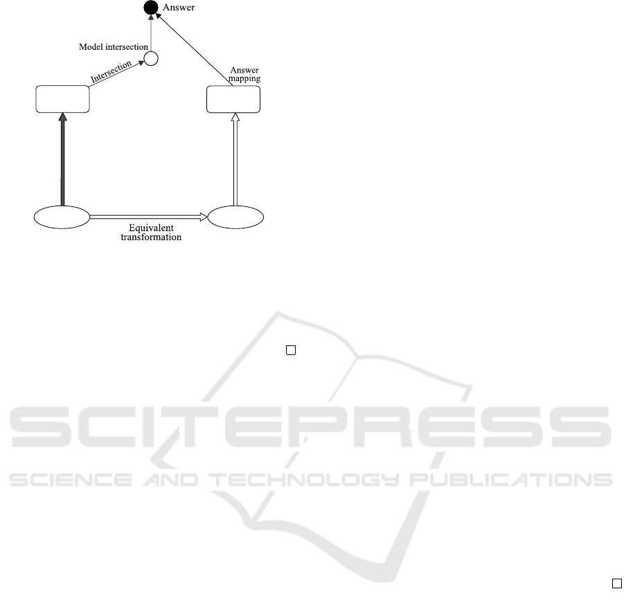
ϕ ϕ
0
S
0
S
0
= hCs, ϕi
S
n
S
n
= hCs
0
, ϕ
0
i
S
0
⇒ S
1
⇒ · · · ⇒ S
n
Models
A
Figure 2: Computation paths are constructed by a combina-
tion of an ET sequence and application of an answer map-
ping.
Definition 4. An ET rule r on STATE is a partial
mapping from STATE to STATE such that for any
S ∈ dom(r), hS,r(S)i is an ET step.
4.4 A Correct Solution Method based
on ET Rules
A MI problem hCs,ϕi, where Cs ⊆ ECLS
F
and ϕ is
an extraction mapping, can be solved as follows:
1. Let A be an answer mapping.
2. Prepare a set R of ET rules on STATE.
3. Take S
0
such that S
0
= hCs,ϕi to start computa-
tion from S
0
.
4. Construct an ET sequence [S
0
,..., S
n
] by applying
ET rules in R, i.e., for each i ∈ {0,1,. .. ,n − 1},
S
i+1
is obtained from S
i
by selecting and applying
r
i
∈ R such that S
i
∈ dom(r
i
) and r
i
(S
i
) = S
i+1
.
5. Assume that S
n
= hCs
n
,ϕ
n
i. If the computation
reaches the domain of A, i.e., hCs
n
,ϕ
n
i ∈ dom(A),
then compute the answer by using the answer
mapping A, i.e., output A(Cs
n
,ϕ
n
).
Given a set Cs of clauses and an extraction map-
ping ϕ, the answer to the MI problem hCs,ϕi is
ϕ(
T
Models(Cs)), which is called the definition path
and is represented by the left path in Fig. 2. The de-
finition path is usually not suitable for computing the
answer since it may take huge cost. Instead of ta-
king this definition path, we take a computation path
consisting of (i) the lowest path (from Cs to Cs
0
)
for ET computation and (ii) the right path (from Cs
0
through the answer mapping A upwards to the answer)
in Fig. 2.
F
1
: ∃x : W (x)
F
2
: ∃x : F(x)
F
3
: ∃x : B(x)
F
4
: ∃x : C(x)
F
5
: ∃x : S(x)
F
6
: ∀x : (W (x) → A(x))
F
7
: ∀x : (F(x) → A(x))
F
8
: ∀x : (B(x) → A(x))
F
9
: ∀x : (C(x) → A(x))
F
10
: ∀x : (S(x) → A(x))
F
11
: ∃x : G(x)
F
12
: ∀x : (G(x) → P(x))
F
13
: ∀x : [A(x) →
[[∀y : (P(y) → E(x, y))] ∨
[∀y : (A(y) ∧ M(y, x) ∧
(∃z : (E(y,z) ∧ P(z))) → E(x,y))]]]
F
14
: ∀x : (C(x) → (∀y : (B(y) → M(x, y))))
F
15
: ∀x : (S(x) → (∀y : (B(y) → M(x,y))))
F
16
: ∀x : (B(x) → (∀y : (F(y) → M(x,y))))
F
17
: ∀x : (F(x) → (∀y : (W (y) → M(x, y))))
F
18
: ∀x : (W (x) → (∀y : ((F(y) ∨ G(y)) → ¬E(x, y))))
F
19
: ∀x : (B(x) → (∀y : (C(y) → E(x, y))))
F
20
: ∀x : (B(x) → (∀y : (S(y) → ¬E(x, y))))
F
21
: ∀x : (C(x) → (∃y : (P(y) ∧ E(x,y))))
F
22
: ∀x : (S(x) → (∃y : (P(y) ∧ E(x, y))))
F
23
: ∃x : [A(x) ∧ [∃y : (A(y) ∧ [∃z : (G(z) ∧ E(y,z))]
∧ E(x,y))]]
Figure 3: Background knowledge represented by first-order
formulas.
The selection of r
i
in R at Step 4 is nondeterminis-
tic and there may be many possible ET sequences for
each MI problem. Every output computed by using
any arbitrary ET sequence is correct.
Theorem 1. Let A be an answer mapping. When an
ET sequence starting from S
0
= hCs,ϕi reaches S
n
in
dom(A), the above procedure gives the correct ans-
wer to hCs,ϕi.
5 A SIMPLE EXAMPLE
5.1 Schubert’s Steamroller Puzzle
The Steamroller puzzle was presented by Lenhart
Schubert in 1978 as a challenge to automated-
deduction systems. It was considered to be too hard
for existing theorem provers at that time due to its big
search space. Much work has been done related to the
Steamroller puzzle to improve efficiency of computa-
tion (Manthey and Bry, 1988; Pelletier, 1986; Stic-
kel, 1986; Walther, 1985; Wang and Bledsoe, 1987).
This is the reason why we take this puzzle in this pa-
per. This example will be used in Section 7 to explain
Computation Control by Prioritized ET Rules
89

computation control with prioritized ET rules and to
illustrate the effect of computation control.
This puzzle is a proof problem. Formalization of
the Steamroller puzzle as a proof problem based on
the conventional theory is given in Section 5.3. Since
proof problems can be transformed into MI problems
according to our theory, we give a formulation of the
Steamroller puzzle as a MI problem in Section 5.4.
5.2 Formalization
The problem description of the Steamroller puzzle
is as follows: Wolves, foxes, birds, caterpillars, and
snails are animals, and there are some of each of them.
Also there are some grains, and grains are plants.
Every animal either likes to eat all plants or all ani-
mals much smaller than itself that like to eat some
plants. Caterpillars and snails are much smaller than
birds, which are much smaller than foxes, which in
turn are much smaller than wolves. Wolves do not
like to eat foxes or grains, while birds like to eat ca-
terpillars but not snails. Caterpillars and snails like
to eat some plants. Therefore there is an animal that
likes to eat a grain-eating animal.
Fig. 3 shows the first-order formulas representing
this problem (Stickel, 1986). The last sentence of the
description (“Therefore there is an animal that likes
to eat a grain-eating animal”) is regarded as a conclu-
sion to be proved and is represented by the first-order
formula F
23
in Fig. 3. All sentences except the last
one form the background knowledge and are repre-
sented by F
1
–F
22
in Fig. 3. This formalization uses
the following predicates as abbreviation:
A(x) – x is an animal W (x) – x is a wolf
F(x) – x is a fox B(x) – x is a bird
C(x) – x is a caterpillar S(x) – x is a snail
G(x) – x is a grain P(x) – x is a plant
M(x,y) – x is much smaller than y
E(x,y) – x likes to eat y
5.3 Clausal Form and A Solution
Referring to F
1
–F
23
in Fig. 3, let F = F
1
∧ F
2
∧ ·· · ∧
F
22
. According to the conventional theory, the Ste-
amroller puzzle is first formalized as a proof problem
F |= F
23
, which is proved by showing that F ∧ ¬F
23
has no model, i.e., Models(F ∧ ¬F
23
) = ∅. By
using conventional Skolemization, F ∧ ¬F
23
is con-
verted into a clause set Cs consisting of the clauses in
Fig. 4, where w, f , b, c, s, and g are Skolem con-
stants, and f
1
and f
2
are Skolem functions. Since
Models(F ∧ ¬F
23
) = Models(Cs), we need to show
that Models(Cs) = ∅. For this purpose the resolution
and factoring inference rules can be used.
C
1
: W (w) ←
C
2
: F( f ) ←
C
3
: B(b) ←
C
4
: C(c) ←
C
5
: S(s) ←
C
6
: G(g) ←
C
7
: A(x) ← W(x)
C
8
: A(x) ← F(x)
C
9
: A(x) ← B(x)
C
10
: A(x) ← C(x)
C
11
: A(x) ← S(x)
C
12
: P(x) ← G(x)
C
13
: E(x,y),E(x,z) ← A(x),P(y),A(z), M(z,x),
P(u),E(z, u)
C
14
: M(x, y) ← C(x),B(y)
C
15
: M(x, y) ← S(x),B(y)
C
16
: M(x, y) ← B(x),F(y)
C
17
: M(x, y) ← F(x),W (y)
C
18
: ← W (x), F(y),E(x, y)
C
19
: ← W (x), G(y),E(x,y)
C
20
: E(x,y) ← B(x),C(y)
C
21
: ← B(x), S(y),E(x,y)
C
22
: P( f
1
(x)) ← C(x)
C
23
: E(x, f
1
(x)) ← C(x)
C
24
: P( f
2
(x)) ← S(x)
C
25
: E(x, f
2
(x)) ← S(x)
C
26
: ← A(x), A(y),G(z),E(y,z),E(x,y)
Figure 4: Clausal form.
5.4 Solving the Puzzle as a MI Problem
This solution is explained in our theory as follows:
The Steamroller puzzle is first formalized as a proof
problem hF,F
23
i, which asks whether F |= F
23
or not.
This is reformalized as a MI problem hF ∧ ¬F
23
,ϕi,
where ϕ is a mapping from pow(G) to {yes,no} such
that for any G ⊆ G, ϕ(G) = “yes” if G = G , ot-
herwise ϕ(G) = “no”. Since Models(F ∧ ¬F
23
) =
Models(Cs), the MI problem hF ∧ ¬F
23
,ϕi is trans-
formed equivalently to a MI problem hCs,ϕi. Many
ET rules are used for solving this MI problem.
6 COMPUTATION WITH
PRIORITIZED ET RULES
6.1 Finite and Infinite Computation
with Prioritized ET Rules
Let R
p
be a sequence of ET rules such that R
p
=
[r
1
,r
2
,..., r
m
]. Let S be a state. Since the rule order
in [r
1
,r
2
,..., r
m
] is used for specifying the priority of
rule application to a state S, R
p
is regarded as a set of
KEOD 2018 - 10th International Conference on Knowledge Engineering and Ontology Development
90

prioritized ET rules.
R
p
is applicable to S with r
j
if
1. none of r
1
,r
2
,..., r
j−1
is applicable to S, and
2. r
j
is applicable to S.
Note that j is determined uniquely by S and R
p
. If R
p
is applicable to S with r
j
, the result of the application
of R
p
to S, denoted by R
p
(S), is r
j
(S).
Given a state S
0
, R
p
determines a finite or infinite
sequence of states as follows:
1. R
p
determines a finite sequence [S
0
,S
1
,..., S
n
] if
(a) R
p
is applicable to S
i
for each i ∈ {0, 1,. .. ,n −
1},
(b) S
i+1
= R
p
(S
i
) for each i ∈ {0, 1,. .. ,n − 1}, and
(c) R
p
is not applicable to S
n
.
2. R
p
determines an infinite sequence [S
0
,S
1
,...] if
(a) R
p
is applicable to S
i
for each i ∈ {0, 1,. ..}, and
(b) S
i+1
= R
p
(S
i
) for each i ∈ {0, 1,. ..}.
Let R
p
= [r
1
,r
2
,..., r
m
] and let A be an answer
mapping. Assume that for any i ∈ {1,2,...,m} and
any state S, if S ∈ dom(A), then r
i
is not applicable
to S. Then, if R
p
produces an infinite computation
[S
0
,S
1
,...], none of S
0
,S
1
,... is in dom(A). We have
the following three cases:
1. If R
p
determines a finite sequence [S
0
,S
1
,..., S
n
],
S
n
∈ dom(A), and S
n
= hCs
n
,ϕ
n
i, then the compu-
ted answer is A(Cs
n
,ϕ
n
).
2. If R
p
determines a finite sequence [S
0
,S
1
,..., S
n
]
and S
n
/∈ dom(A), then no answer is obtained.
3. If R
p
determines an infinite sequence [S
0
,S
1
,...],
then no answer is obtained.
6.2 Correctness of Computation with
Prioritized ET Rules
Given a set Cs of extended clauses and an extraction
mapping ϕ, the MI problem hCs, ϕi can be solved as
follows:
1. Let A be an answer mapping.
2. Prepare a sequence R
p
of ET rules on STATE.
3. Take S
0
such that S
0
= hCs,ϕi to start computa-
tion from S
0
.
4. Assume that R
p
determines a finite sequence
[S
0
,S
1
,..., S
n
] and S
n
= hCs
n
,ϕ
n
i.
5. If the computation reaches the domain of A,
i.e., hCs
n
,ϕ
n
i ∈ dom(A), then compute the ans-
wer by using the answer mapping A, i.e., output
A(Cs
n
,ϕ
n
).
The selection of R
p
is arbitrary and there are
many possible computation paths depending on the
selection of ET rules in R
p
and the order of them in
R
p
. Every output computed by using any arbitrary
computation path is correct.
Theorem 2. When an ET sequence starting from S
0
=
hCs,ϕi reaches S
n
in dom(A), the above procedure
gives the correct answer to hCs, ϕi.
Proof: Since [S
0
,S
1
,..., S
n
] is an ET sequence,
ans
MI
(Cs,ϕ) = ans
MI
(Cs
n
,ϕ
n
). Since A is an ans-
wer mapping, ans
MI
(Cs
n
,ϕ
n
) = A(Cs
n
,ϕ
n
). Hence
ans
MI
(Cs,ϕ) = A(Cs
n
,ϕ
n
).
7 COMPUTATION CONTROL
WITH PRIORITIZED ET RULES
7.1 Resource Minimization by
Prioritized ET Rules
In practical problem solving, resource for computa-
tion is limited. Typically, we minimize execution time
to reach a conclusion under space constraints. For
each state S = hCs,ϕi,
• the number of clauses in Cs should not exceed a
certain limit, and
• the number of all atoms in Cs should also not ex-
ceed a certain limit.
Assuming that smaller amount of space consumption
tends to decrease total execution time, we will design
a set of ET rules and their priority.
7.2 Restricted Resolution and
Restricted Factoring
Resolution adds a resolvent of two clauses and always
increases the number of clauses by one. Let (res i)
be defined as an ET rule for making a resolution step
with a resolvent containing not more than i atoms.
Since a smaller number atoms are better for saving
space and for finding simpler clauses, the priority or-
der of (res 0),(res 1),(res 2),... is given by:
(res 0) > (res 1) > (res 2) > · ··
Factoring also adds a clause; it always increases
the number of clauses by one. Let (fac i) be de-
fined as a factoring rule with a new clause contai-
ning not more than i atoms. Again, for finding sim-
pler clauses and saving space, the priority order of
(fac 1),(fac 2),(fac 3),.. . is specified by:
(fac 1) > (fac 2) > (fac 3) > ···
Computation Control by Prioritized ET Rules
91

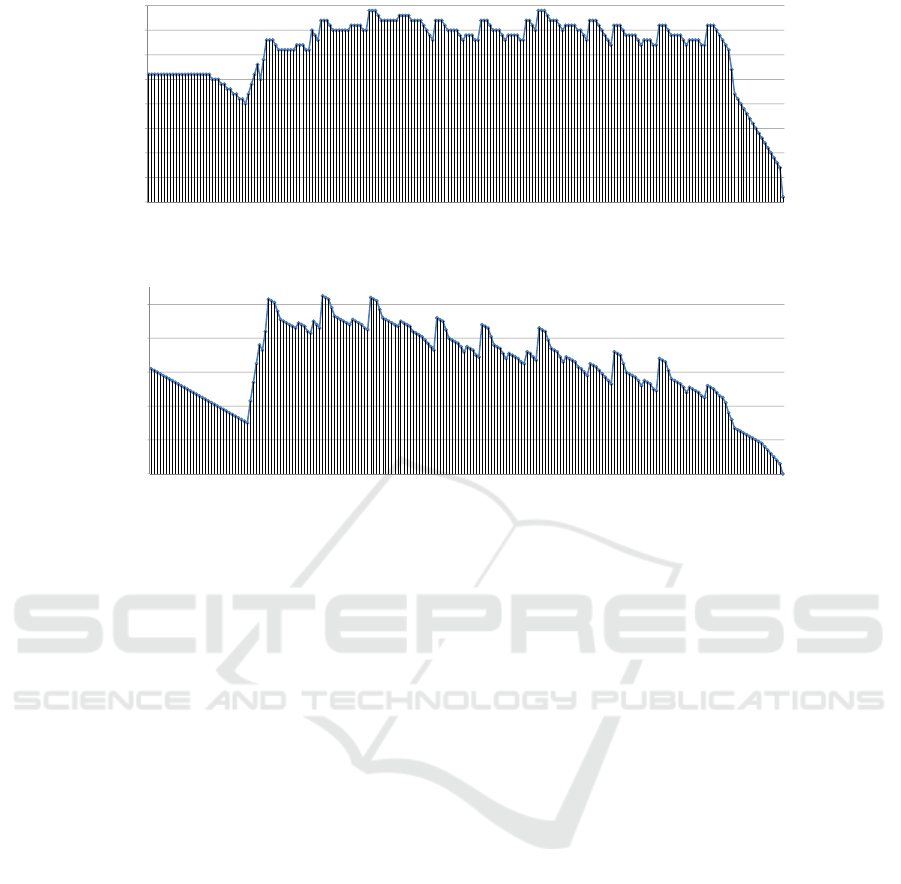
15
20
25
30
35
40
N0. of clauses
0
5
10
1
4
7
10
13
16
19
22
25
28
31
34
37
40
43
46
49
52
55
58
61
64
67
70
73
76
79
82
85
88
91
94
97
100
103
106
109
112
115
118
121
124
127
130
133
136
139
142
145
148
151
154
157
160
163
166
169
172
175
178
181
184
187
190
193
196
199
202
205
208
211
No. of transformation steps
Figure 5: Changes of the number of clauses.
40
60
80
100
Number of atoms
0
20
1
4
7
10
13
16
19
22
25
28
31
34
37
40
43
46
49
52
55
58
61
64
67
70
73
76
79
82
85
88
91
94
97
100
103
106
109
112
115
118
121
124
127
130
133
136
139
142
145
148
151
154
157
160
163
166
169
172
175
178
181
184
187
190
193
196
199
202
205
208
211
Number of transformation steps
Figure 6: Changes of the number of atoms.
7.3 Restricted Unfolding
Unfolding decreases the number of clauses by one
when the number of resolvents is zero, does not
change the number of clauses when it produces only
one resolvent, and increases the number of clauses ot-
herwise.
Unfolding with not more than i resolvents is a
transformation rule that satisfies the following con-
ditions:
1. Letting D be a set of definite clauses used for un-
folding, this rule is applicable to a body atom b in
Cs with respect to Cs and D when
|{C | (C ∈ D) & (b and head(C) is unifiable)}| ≤ i.
2. The result of the transformation is the same as that
of usual unfolding.
Let (udi i) be defined as a transformation rule such
that
• definite-clause removal (see Section 8.2) is app-
lied if it is applicable,
• otherwise unfolding with not more than i resol-
vents is applied if it is applicable.
The priority order of (udi 1), (udi 2),(udi 3), .. . is gi-
ven by:
(udi 1) > (udi 2) > (udi 3) > · ··
7.4 A Solution to the Steamroller
Problem
Let (erase) be an ET rule for erasing independent
satisfiable atoms (see Section 8.5), (subsumed) an
ET rule for elimination of subsumed clauses (see
Section 8.6), and (fwd) an ET rule for forwarding
transformation. When we take the rule priority
(udi 1) > (erase) > (subsumed) >
(fwd) > (udi 2) > (udi 3) > (udi 5),
the Steamroller puzzle is solved by 211 rule applica-
tions. Changes of the number of clauses and those
of the number of atoms are shown by Fig. 5 and
Fig. 6, respectively, where (udi 1) is applied 116 ti-
mes, (erase) 15 times, (subsumed) 38 times, (fwd) 17
times, (udi 2) 8 times, (udi 3) 4 times, and (udi 5) 13
times.
7.5 Comparison
By deleting (udi 2) and (udi 3) from the above priority,
we have
(udi 1) > (erase) > (subsumed) > (fwd) > (udi 5),
which gives only 90 steps to obtain the same solution.
However, when we remove the rule (udi 1), i.e., when
we take
(erase) > (subsumed) > (fwd) > (udi 5),
KEOD 2018 - 10th International Conference on Knowledge Engineering and Ontology Development
92

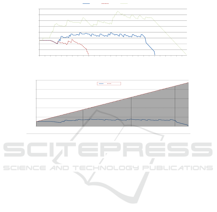
0
10
20
30
40
50
60
70
80
1 11 21 31 41 51 61 71 81 91 101 111 121 131 141 151 161 171 181 191 201 211 221 231 241251261
No. of clauses
No. of transformation steps
Cont01 Cont02 Cont03
Figure 7: Computation control comparison.
100
150
200
250
No. of clauses
ET
Resolution
0
50
1
4
7
10
13
16
19
22
25
28
31
34
37
40
43
46
49
52
55
58
61
64
67
70
73
76
79
82
85
88
91
94
97
100
103
106
109
112
115
118
121
124
127
130
133
136
139
142
145
148
151
154
157
160
163
166
169
172
175
178
181
184
187
190
193
196
199
202
205
208
211
No. of clauses
No. of transformation steps
Figure 8: Comparing computation by ET with that by resolution and factoring.
we need 269 steps to reach the final singleton of the
empty clause, showing that prioritized application of
(udi 1) is important for efficient computation.
So far we have introduced three priority controls,
which are referred to as “Cont01”, “Cont02”, and
“Cont03”. Changes of the number of clauses resulting
from these priority controls when solving the Steam-
roller puzzle are shown in Fig 7.
Since resolution and factoring are ET rules, the
conventional resolution proof method is covered by
our framework. For example, we can take prioritized
ET rules (res 99) > (fac 99) to solve proof problems
by the resolution and factoring ET rules.
Fig. 8 compares ET computation using the priority
control “Cont01” with computation by resolution and
factoring. Since each resolution step adds one resol-
vent of two clauses, each step increases the number of
clauses by one. In the proof with resolution and facto-
ring, computation goes on the upward straight line in
Fig. 8, which may exceed the space limitation before
the computation terminates.
7.6 Efficiency Improvement
Our method has a chance to improve efficiency com-
pared to the conventional resolution-based methods.
All strategies taken in the resolution-based methods
can also be used in our theory. Adoption of new ET
rules and adjustment of rule priority provide a power-
ful mechanism for computation control, which cannot
be utilized in the conventional methods.
It is expected that the method of prioritized ET ru-
les overcomes the limitation of the conventional met-
hods, since we can plan to search goals with unlimi-
ted variety of ET rules. So far, this has been experi-
mentally shown by several small proof problems and
QA problems, such as the Agatha proof problem (with
built-in atoms) and the Agatha QA problem (Akama
and Nantajeewarawat, 2018b).
8 ET RULES BY EXAMPLES
In this section we explain the ET rules used in this
paper by examples. Their strict mathematical defi-
nitions and correctness proofs can be found elsew-
here (Akama and Nantajeewarawat, 2016b; Akama
and Nantajeewarawat, 2018a).
8.1 Unfolding
Unfolding with respect to an atom b for extended
clauses on ECLS
F
is the same as unfolding for usual
clauses except the possible avoidance of application
such as existence of multi-head clauses containing b
in their head parts.
Computation Control by Prioritized ET Rules
93

For instance, suppose that Cs contains the four
clauses:
C
1
: p
1
← p
2
, p
3
C
2
: p
1
← p
4
C
3
: p
1
, p
2
← p
5
C
4
: h
1
,h
2
← p
1
, p
6
Then C
4
cannot be unfolded at p
1
since p
1
belongs to
the head part of the multi-head clause C
3
.
8.2 Definite-Clause Removal
Useless definite clauses with respect to unfolding are
removed by this rule. For instance, consider a MI pro-
blem hCs, ϕi. Assume that ϕ does not depend on p
1
and Cs consists of the following clauses:
C
1
: p
1
← p
2
, p
3
C
2
: p
1
← p
4
C
3
: p
8
← p
2
C
4
: h
1
,h
2
← p
6
, p
8
Then C
1
and C
2
can be removed from Cs since p
1
does
not appear in the right-hand side of any other clause
in Cs.
8.3 Resolution
Resolution for extended clauses on ECLS
F
is the
same as resolution for usual clauses except the pos-
sible existence of func-atoms. Only usual variables in
func-atoms are changed by the most general unifier in
use; function variables are not changed.
For instance, suppose that Cs contains the two
clauses:
C
1
: p(x) ← q(x),r(x,4),s(x),func(h,x)
C
2
: r(1,y),t(y,z) ← u(y),v(z)
By applying the resolution rule to C
1
and C
2
, a new
clause
C
3
: p(1),t(4,z) ← q(1),s(1), u(4),v(z), func(h,1)
is added to Cs as the resolvent.
8.4 Factoring
Two atoms in the same side in a clause are unified
to give a new clause. For instance, suppose that Cs
contains the clause:
C
1
: p(x) ← q(x),r(x,4),r(3,y),func(h, y)
Then a new clause
C
2
: p(3) ← q(3),r(3,4), func(h,4)
is added to Cs. Suppose that Cs contains the clause:
C
3
: p(x), r(x,4),r(3,y) ← func(h,y)
A new clause
C
4
: p(3), r(3,4) ← func(h, 4)
is added.
8.5 Erasing Independent Satisfiable
Atoms
Let C be a clause and B a set of atoms. Let C  B
be defined as the clause obtained from C by remo-
ving all atoms in B from its right-hand side. That
is, C  B is defined by lhs(C  B) = lhs(C) and
rhs(C  B) = rhs(C) − B. This rule, referred to as
(erase) in Section 7, changes C into C  B if (i) B and
(lhs(C) ∪ rhs(C)) − B have no common variable and
(ii) B can be instantiated to be true under the condition
of Cs − {C}.
For instance, suppose that Cs contains the two
clauses:
C
1
: p( f (2,6)) ←
C
2
: r(y) ← p( f (x,6)), q(y)
Then p( f (x,6)) can be removed from C
2
.
8.6 Elimination of Subsumed Clauses
This rule, referred to as (subsumed) in Section 7, re-
moves a clause C from a clause set Cs if C is subsu-
med by some clause in Cs. For instance, suppose that
Cs contains the two clauses:
C
1
: h
1
,h
2
← b
1
,b
2
C
2
: h
1
← b
2
Then C
1
can be removed from Cs.
9 CONCLUSIONS
Model-intersection (MI) problems constitute one of
the largest classes of logical problems. Proof pro-
blems and QA problems on first-order logic can be
solved by transforming them into MI-problems on ex-
tended clauses and by searching paths to target sets
of extended clauses. We take extended clauses in
ECLS
F
, which overcomes the serious limitation of ex-
pressive power of conventional clauses, where exis-
tential quantification is never represented.
An ET rule is a partial mapping on the powerset of
ECLS
F
that preserves the answer to a given MI pro-
blem. Most ET rules transform a clause set Cs preser-
ving Models(Cs) and/or
T
Models(Cs). The possibi-
lity of using ET rules unlimitedly has fundamentally
changed the concept of computation. The conventio-
nal concept of computation in logical problem solving
is based on procedural reading of logical formulas,
while computation in our theory is successive appli-
cation of an unlimited number of ET rules, which are
not logical formulas. Correctness of computation by
ET rules has been strictly guaranteed.
KEOD 2018 - 10th International Conference on Knowledge Engineering and Ontology Development
94

On the basis of such fundamental changes of the
computation framework, a new concept of computa-
tion control has been introduced in this paper. Ap-
plication priority among ET rules works as compu-
tation control. Priority ordering in a set of ET rules
limits computation variety. Appropriate selection of
priority ordering is useful for finding efficient com-
putation paths.
1
Many conventional methods for lo-
gical computation use restricted sets of ET rules and
restricted control within the ET rules, and can be re-
garded as special forms of our method. It is expected
that prioritized ET rules will produce more efficient
solutions for logical problem solving.
ACKNOWLEDGEMENTS
This research was partially supported by JSPS KA-
KENHI Grant Numbers 25280078 and 26540110.
REFERENCES
Akama, K. and Nantajeewarawat, E. (2011). Meaning-
Preserving Skolemization. In Proceedings of the 3rd
International Conference on Knowledge Engineering
and Ontology Development, pages 322–327, Paris,
France.
Akama, K. and Nantajeewarawat, E. (2016a). Model-
Intersection Problems with Existentially Quantified
Function Variables: Formalization and a Solution
Schema. In Proceedings of the 8th International Joint
Conference on Knowledge Discovery, Knowledge En-
gineering and Knowledge Management (IC3K 2016),
Volume 2: KEOD, pages 52–63, Porto, Portugal.
Akama, K. and Nantajeewarawat, E. (2016b). Unfolding
Existentially Quantified Sets of Extended Clauses.
In Proceedings of the 8th International Joint Confe-
rence on Knowledge Discovery, Knowledge Engineer-
ing and Knowledge Management (IC3K 2016), Vo-
lume 2: KEOD, pages 96–103, Porto, Portugal.
Akama, K. and Nantajeewarawat, E. (2018a). Computation
Control by Prioritized ET Rules. Technical report, In-
formation Initiative Center, Hokkaido University.
Akama, K. and Nantajeewarawat, E. (2018b). Sol-
ving Query-Answering Problems with Constraints for
Function Variables. In Proceedings of the 10th Asian
Conference on Intelligent Information and Database
Systems, LNAI 10751, pages 36–47, Dong Hoi City,
Vietnam.
Manthey, R. and Bry, F. (1988). SATCHMO: A Theo-
rem Prover Implemented in Prolog. In Proceedings
1
The current version of our MI solver receives a problem
description and control priority as input and produces an ET
sequence and the final answer (when the computation rea-
ches it), where finding good computation control is essential
for the success of solving problems in practical time.
of the 9th International Conference on Automated De-
duction, LNCS 310, pages 415–434, Argonne, IL.
Pelletier, F. J. (1986). Seventy-Five Problems for Testing
Automatic Theorem Provers. Journal of Automated
Reasoning, 2(2):191–216.
Stickel, M. (1986). Schubert’s Steamroller Problem: For-
mulations and Solution. Journal of Automated Reaso-
ning, 2(2):89–104.
Walther, C. (1985). A Mechanical Solution of Schubert’s
Steamroller by Many-Sorted Resolution. Artificial In-
telligence, 26(2):217–224.
Wang, T.-C. and Bledsoe, W. W. (1987). Hierarchical De-
duction. Journal of Automated Deduction, 3(1):35–
77.
Computation Control by Prioritized ET Rules
95