
Approximate Recursive Bayesian Estimation of State
Space Model with Uniform Noise
Lenka Pavelkov
´
a and Ladislav Jirsa
Institute of Information Theory and Automation, The Czech Academy of Sciences, Pod Vod
´
arenskou v
ˇ
e
ˇ
z
´
ı 4,
Prague, Czech Republic
Keywords:
State Estimation, State-space Models, Linear Systems, Bounded Noise, Probabilistic Models, Approximate
Estimation, Recursive Estimation.
Abstract:
This paper proposes a recursive algorithm for the state estimation of a linear stochastic state space model.
A model with discrete-time inputs, outputs and states is considered. The model matrices are supposed to
be known. A noise of the involved model is described by a uniform distribution. The states are estimated
using Bayesian approach. Without using an approximation, the complexity of the posterior probability density
function (pdf) increases with time. The paper proposes an approximation of this complex pdf so that a feasible
support of the posterior pdf is kept during the estimation. The state estimation consists of two stages, namely
the time and data update including the mentioned approximation. The behaviour of the proposed algorithm is
illustrated by simulations and compared with other methods.
1 INTRODUCTION
A state space model is frequently used for a descrip-
tion of real systems. The unobserved states are es-
timated using measured data, i. e., system inputs
and outputs, as well as modelled dependencies among
particular states. Uncertainties of a state evolution
model and of an observation model are often sup-
posed to have normal distribution. Then, the states
are standardly estimated by means of Kalman filtering
(KF) (Jazwinski, 1970) and its extensions. However,
the unbounded support of the Gaussian distribution
can cause difficulties if the estimated quantity is phys-
ically bounded as, for instance, it may give unreason-
able negative estimates of naturally non-negative vari-
able. There are several ways to deal with this case.
In the KF framework, the state estimates can be
projected onto the constraint surface via quadratic
programming (Fletcher, 2000) or the Gaussian distri-
bution is truncated (Simon and Simon, 2010).
A robust recursive Kalman-like algorithm for the
state estimation of linear models with disturbances
bounded by ellipsoids is proposed in (Becis-Aubry
et al., 2008). The proposed algorithm consists of two
steps: time updating and observation updating.
A zonotopic Kalman filter (ZKF) is proposed in
(Combastel, 2015). Discrete-time LTV/LPV systems
with state and measurement uncertainties are con-
sidered. ZKF computes minimal zonotopic sets en-
closing all the admissible states. Explicit links be-
tween the zonotopic set-membership and the stochas-
tic paradigms for Kalman filtering are given.
The papers (Lang et al., 2007) and (Shao et al.,
2010) investigate constrained Bayesian state estima-
tion problems by using a particle filter (PF) approach.
In these papers, algorithms are proposed. inequality
constraints are imposed by accept/reject steps in the
algorithms. The Monte-Carlo methods require, how-
ever, a huge amount of samples to obtain acceptable
results.
In the paper (Dabbene et al., 2014), a rapproche-
ment between the stochastic and worst-case system
identification viewpoints is presented. There, the so-
called worst-case radius of information is decreased at
the expense of a given probabilistic “risk”. A case of
uniformly distributed noise is supposed. A trade-off
curve is constructed which shows how the radius of
information decreases as a function of the accuracy.
In the paper (Chisci et al., 1996), the prob-
lem of recursively estimating the state of a discrete-
time linear dynamical system subject to bounded
disturbances is addressed. An approach based on
minimum-volume bounding parallelotopes is intro-
duced and an algorithm of polynomial complexity
is derived. The estimates are intended in a “set-
membership” sense. In (Pavelkov
´
a and K
´
arn
´
y, 2014),
388
Pavelková, L. and Jirsa, L.
Approximate Recursive Bayesian Estimation of State Space Model with Uniform Noise.
DOI: 10.5220/0006933803880394
In Proceedings of the 15th International Conference on Informatics in Control, Automation and Robotics (ICINCO 2018) - Volume 1, pages 388-394
ISBN: 978-989-758-321-6
Copyright © 2018 by SCITEPRESS – Science and Technology Publications, Lda. All rights reserved

joint parameter and state estimation is proposed for
linear state-space model with uniform state and out-
put noises. The proposed approximate Bayesian es-
timator provides the maximum a posteriori estimate
enriched by information on its precision without de-
manding the user to tune noise covariances.
Inspired by (Combastel, 2015) and (Chisci et al.,
1996), we extend our previous results of an ap-
proximate Bayesian estimation for regressive model
(Pavelkov
´
a and Jirsa, 2017) to the state space model
and propose an estimator that provides a state estimate
of a linear state-space model with a uniform noise.
We use Bayesian filtration applied to uniform pdfs.
The approach is probabilistic, the method explicitly
operates on pdfs using the general theory. The sim-
ple recursive algorithm gives a probabilistic estimate
that is kept in a given class of functions. The approx-
imate posterior probability function has a parallelo-
topic support.
Throughout the paper, the following notation will
be used: z
t
is the value of a column vector z at
a discrete-time instant t ∈ t
?
≡ {1, 2, ... ,t}; z
t;i
is the
i-th entry of z
t
; `
z
is the length of the vector z; z and
z are lower and upper bounds on z, respectively; ≡
means equality by the definition, ∝ means equality up
to a constant factor. The symbol f (·|·) denotes a con-
ditional probability density function (pdf); names of
arguments distinguish respective pdfs; no formal dis-
tinction is made between a random variable, its real-
isation and an argument of the pdf. U
z
(z,z) denotes
the uniform pdf of z with support [z,z].
2 ADDRESSED PROBLEM
A controlled system can be described by the set of `
y
-
dimensional observable outputs y
t
, of `
u
-dimensional
system inputs u
t
, and `
x
-dimensional unobservable
system states x
t
, t ∈ t
?
≡ {1,2,. .. ,t}. The input-
output pair is called data, i.e. d
t
= (u
t
,y
t
).
In the considered Bayesian set up (K
´
arn
´
y et al.,
2005), the system is modelled by pdfs. Using the
chain rule and considering the independent input se-
quence u
0
,u
1
,. .. ,u
t−1
, the joint pdf of all involved
variables, f (d
1
, . .. , d
t
,x
0
, . .. , x
t
), can be factorised
to the product of factors (1). Note that we use a
different factorisation comparing to (K
´
arn
´
y et al.,
2005). There, the time evolution model has the form
f (x
t
|
x
t−1
,u
t
).
We factorise the joint pdf as follows
f (d
1
, . .. , d
t
,x
0
, . .. , x
t
) = (1)
= f (x
0
)
|{z}
prior pdf
t
∏
t=1
f (u
t
)
|{z}
input generator
×
×
t
∏
t=1
f (y
t
|
x
t
)
| {z }
observation model
f (x
t
|
x
t−1
,u
t−1
)
| {z }
time evolution model
.
The resulting form assumes that (i) state x
t
satis-
fies Markov property and (ii) no direct relationship
between input and output exists in the observation
model.
The Bayesian state estimation or filtering (K
´
arn
´
y
et al., 2005) consists in the evolution of the posterior
pdf f (x
t
|d(t)), d(t) ≡ {d
1
, d
2
, . .. , d
t
} is a sequence
of observed data records d
t
= (y
t
,u
t
), t ∈ t
?
, d
0
≡ u
0
.
The evolution of f (x
t
|d(t)) is described by the recur-
sion that starts from the prior pdf f (x
0
|d(0)) ≡ f (x
0
):
• Time update
f (x
t
|d(t −1)) =
Z
x
?
t−1
f (x
t
|u
t−1
,x
t−1
) f (x
t−1
|d(t −1)) dx
t−1
(2)
that reflects the time evolution x
t−1
→ x
t
and
• Data update
f (x
t
|d(t)) =
f (y
t
|x
t
) f (x
t
|d(t − 1))
f (y
t
|d(t − 1))
=
=
f (y
t
|x
t
) f (x
t
|d(t − 1))
R
x
?
t−1
f (y
t
|x
t
) f (x
t
|d(t − 1))dx
t−1
(3)
that incorporates information about data d
t
.
Here, we focus on a linear model state space
model in the form
x
t
= Ax
t−1
+ Bu
t−1
| {z }
˜x
t
+ν
t
, ν
t
∼ U
ν
(−ρ,ρ)
y
t
= Cx
t
|{z}
˜y
t
+n
t
, n
t
∼ U
n
(−r, r)
(4)
where A, B, C are the known model matrices of appro-
priate dimensions, ν
t
∈ (−ρ, ρ) is the uniform state
noise, n
t
∈ (−r, r) is the uniform output noise.
Equivalently, using pdf notation
f (x
t
|u
t−1
,x
t−1
) = U
x
( ˜x
t
− ρ, ˜x
t
+ ρ) (5)
f (y
t
|x
t
) = U
y
( ˜y
t
− r, ˜y
t
+ r).
State estimation of (5) according to (2) and (3)
leads to a very complex form of posterior pdf. This
paper proposes an approximate Bayesian state esti-
mation of the linear state space model with uniform
noise (LSU model) (4) where the posterior pdf is uni-
formly distributed on a parallelotopic support.
Approximate Recursive Bayesian Estimation of State Space Model with Uniform Noise
389

3 ALGORITHMIC SOLUTION
Here, the approximate state estimation of model (5)
is proposed. The presented algorithm provides the
evolution of the approximate posterior pdf f (x
t
|d(t)).
The proposed algorithm needs a knowledge about the
noise bounds ρ and r in (5). These bounds are gen-
erally unknown. To obtain their estimates, the algo-
rithm as proposed by author in (Pavelkov
´
a and K
´
arn
´
y,
2014) can be used. It provides the point estimates of
respective noise bounds of (5).
3.1 Approximate Time Update
3.1.1 Exact Computation
The time update according to (2) starts at t = 1 with
f (x
t−1
|d(t − 1)) = f (x
0
). We suppose that the prior
pdf f (x
0
) is uniform on an orthotopic support,
f (x
0
) = U
x
0
(x
0
,x
0
). (6)
In the next steps, without approximation, the prior
pdf f (x
t−1
|d(t − 1)) would be generally non-uniform
with a polytopic support. The below proposed
double approximation keeps the uniform orthotopic
form of f (x
t−1
|d(t − 1)), i.e. f (x
t−1
|d(t − 1)) =
U
x
t−1
(x
t−1
, x
t−1
). Then, (2) gives
f (x
t
|d(t − 1)) =
=
Z
x
?
t−1
U
x
t
( ˜x
t−1
− ρ, ˜x
t−1
+ ρ)U
x
t−1
(x
t−1
, x
t−1
)dx
t−1
=
=
1
|
det(A)
|
`
x
∏
i=1
1
2ρ
i
(x
t−1;i
− x
t−1;i
)
× (7)
×
`
x
∏
i=1
([(x
t;i
− B
i
u
t−1
+ ρ
i
)χ(x
t;i
< B
i
u
t−1
+ m
t;i
− ρ
i
) +
+m
t;i
χ(x
t;i
≥ B
i
u
t−1
+ m
t;i
− ρ
i
)]−
−
m
t;i
χ(x
t
;i ≤ B
i
u
t−1
+ m
t;i
+ ρ
i
) +
+(x
t;i
− B
i
u
t−1
− ρ
i
)χ(x
t;i
> B
i
u
t−1
+ m
t;i
+ ρ
i
)
×
×
`
x
∏
i=1
χ(m
t;i
+ B
i
u
t−1
− ρ
i
≤ x
t;i
≤ m
t;i
+ B
i
u
t−1
+ ρ
i
),
| {z }
Cutting according to the conditions given by state evolution model.
where
m
t;i
=
`
x
∑
j=1
min(A
i j
x
t−1; j
,A
i j
x
t−1; j
), (8)
m
t;i
=
`
x
∑
j=1
max(A
i j
x
t−1; j
,A
i j
x
t−1; j
),
A
i j
means the term on the i-th row and the j-th column
of A. The resulting pdf (7) is trapezoidal.
3.1.2 Approximation
We propose an approximation of the original distri-
bution (7) by a uniform distribution. In (Bernardo,
1979), it is shown that an optimal approximation
(in a Bayesian sense) of a pdf by another pdf is
achieved by minimisation of Kullback-Leibler diver-
gence (KLD) (Kullback and Leibler, 1951) of these
two pdfs. If the approximate pdf is uniform, it keeps
the support of the original pdf, see proof in Ap-
pendix A.1. Then,
f (x
t
|d(t − 1)) ≈
≈
`
x
∏
i=1
χ(B
i
u
t−1
+ m
t;i
− ρ
i
≤ x
t;i
≤ B
i
u
t−1
+ m
t;i
+ ρ
i
)
m
t;i
− m
t;i
+ 2ρ
i
=
=
`
x
∏
i=1
U
x
t;i
(B
i
u
t−1
+ m
t;i
− ρ
i
,B
i
u
t−1
+ m
t;i
+ ρ
i
) =
= U
x
t
(Bu
t−1
+ m
t
− ρ, Bu
t−1
+ m
t
+ ρ), (9)
where m
t
= [m
t;1
,. .. , m
t;`
x
]
0
, m
t
= [m
t;1
,. .. , m
t;`
x
]
0
,
i = 1, . . ., `
x
are defined by (8).
3.2 Approximate Data Update
3.2.1 Exact Computation
In this step, both u
t
and y
t
are included. After the
data update according to (3), we obtain a posterior pdf
with a support in the form of polytope. This polytope
results from the intersection of an orthotope obtained
during time update and strips given by new data. For
details see Appendix A.2. It holds
f (x
t
|d(t)) =
1
I
t
U
y
t
(Cx
t
− r,Cx
t
+ r)×
×U
x
t
(Bu
t−1
+ m
t
− ρ, Bu
t−1
+ m
t
+ ρ) (10)
with
I
t
=
Z
x
?
t
U
y
(Cx
t
− r,Cx
t
+ r)×
×U
x
t
(Bu
t−1
+ m
t
− ρ, Bu
t−1
+ m
t
+ ρ)dx
t
.
3.2.2 Approximation
We propose an approximation of (10) by a uniform
distribution on a parallelotope. For this purpose, we
adapt the algorithm from (Vicino and Zappa, 1996).
It holds
f (x
t
|d(t)) ∝
∝ χ(Bu
t−1
+ m
t
− ρ ≤ x
t
≤ Bu
t−1
+ m
t
+ ρ)×
×χ(Cx
t
− r ≤ y
t
≤ Cx
t
+ r) =
=
`
x
∏
i=1
χ(B
i
u
t−1
+ m
t;i
− ρ
i
≤ x
t;i
≤ B
i
u
t−1
+ m
t;i
+ ρ
i
)×
ICINCO 2018 - 15th International Conference on Informatics in Control, Automation and Robotics
390

×
`
y
∏
j=1
χ(y
t; j
− r
j
≤ C
j
x
t
≤ y
t; j
+ r
j
) (11)
where C
j
is j-th row of the matrix C. The approxi-
mated pdf has the form (see Appendix A.2)
f (x
t
|d(t)) ≈ K
t
χ(x
t
≤ M
t
x
t
≤ x
t
), (12)
where K
t
is a normalising constant.
The resulting posterior pdf (12) has a uniform dis-
tribution on a parallelotopic support. The time up-
date (7) in the next step assumes pdf with an ortho-
topic support, i.e. f (x
t
|d(t)) = U
x
t
(x
t
, x
t
). There-
fore, we use “orthotopic” bounds of x
t
. These bounds
are obtained by circumscription of the parallelotope
x
t
≤ M
t
x
t
≤ x
t
in (12), see Appendix A.3. Then
x
t
≤ x
t
≤ x
t
. (13)
In this way, the recursion is closed and the ob-
tained orthotopic bounds (13) can be used in the next
time update step (7) for the computation of the terms
m and m (8).
3.3 Point Estimates
State point estimate corresponds to the centre of sup-
port parallelotope which is identical to the centre of
circumscribing orthotope (Coxeter, 1973). Therefore,
ˆx
t
=
x
t
+ x
t
2
. (14)
Note: Approximation of the posterior pdf (12) on
the parallelotopic support by (13) on the orthotopic
support, that enters the next time step as the prior
pdf preserving the point estimate (14), increases the
pdf support, which increases the state uncertainty and
plays the role of forgetting.
3.4 Algorithmic Summary
Here, the state estimation of model (5) considering
known ρ, r is summarised.
Initialisation:
• Choose final time t > 0, set initial time t = 0
• Determine x
0
, x
0
, u
0
On-line
(i) Set t = t +1
(ii) Compute m
t
, m
t
according to (8)
(iii) Perform data update according to (11)
(iv) Approximate the set x
?
t
by a parallelotope to ob-
tain the form (12) — successive intersections of
parallelotope (orthotope) with the strips given
by individual rows of output equation and the
following approximation by parallelotope (the
algorithm in (Vicino and Zappa, 1996))
(v) Compute x
t
, x
t
(13)
(vi) Compute the point estimate ˆx
t
(14)
(vii) If t < t, go to (i)
4 ILLUSTRATIVE EXAMPLE
In this section, the simulative experiments demon-
strate the proposed algorithm properties. The algo-
rithm is also compared with the zonotopic Kalman fil-
ter (Combastel, 2015), outlined in Section 1, as a sim-
ilar method with adjustable geometrical complexity.
4.1 Experiment Setup
The matrices of the state space model (4) are set as
A =
1.0 −0.5 0.2
0.5 0.1 0.0
0.3 0.0 −0.1
, B =
0.1
0.6
0.3
,
C =
1.0 0.0 0.5
0.0 1.0 0.5
,
ρ
r
=
0.1
0.3
. (15)
Input is randomly generated as u
t
∼ N (0, 1). Length
of data sequences t = 100.
4.2 Results
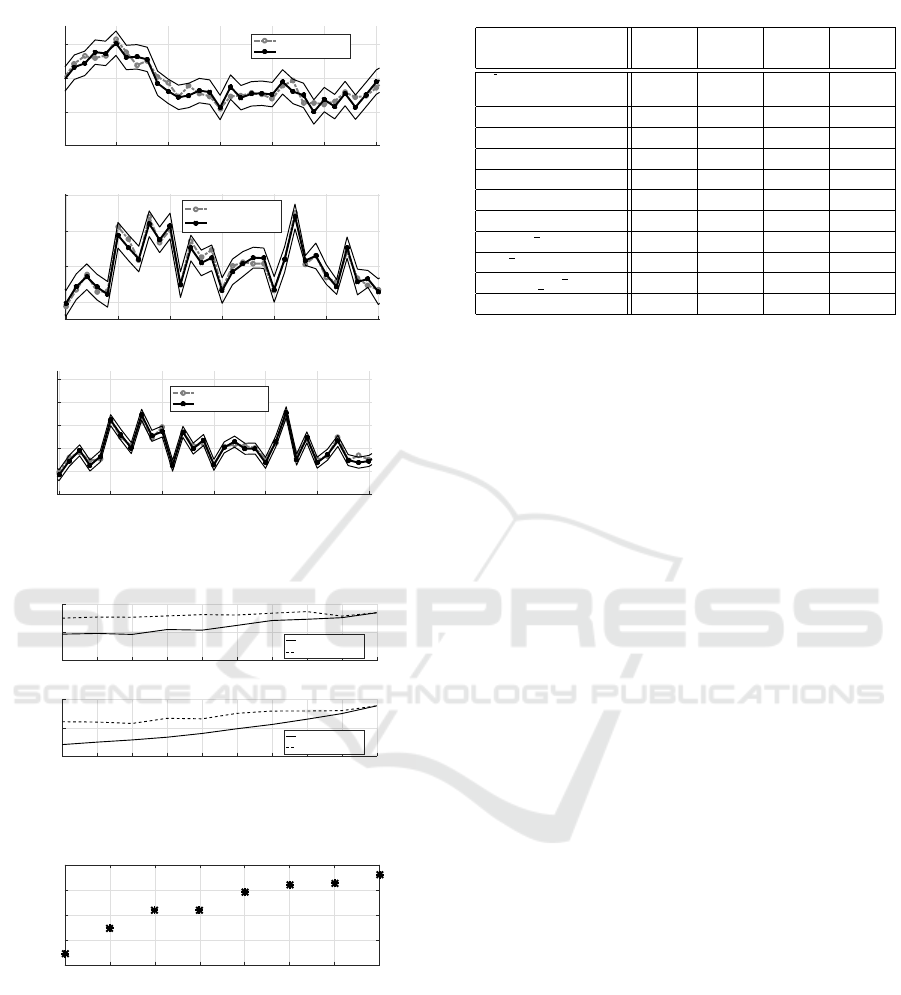
Example of simulated and estimated states together
with the orthotopic bounds (13) is shown in Figure 1,
that is zoomed to demonstrate a typical behaviour.
Figure 2 shows sensitivity of the algorithm to values
of state (ρ) and output (r) noise parameters, examined
on the state x
t;2
. Finally, Figure 3 shows dependence
of execution time on the state dimension.
The proposed algorithm (called LSU) was com-
pared to estimation on a moving window (Pavelkov
´
a
and K
´
arn
´
y, 2014) (WIN, previously developed by the
author) and the zonotopic Kalman filter (Combastel,
2015) (ZKF), see Table 1. Median as a statistic shows
the difference more significantly than the mean. Value
of q denotes the order of zonotope (for q = 3 ≡ `
x
,
a zonotope of order `
x
in an `
x
-dimensional space is
a parallelotope), t runs from 1 to t.
4.3 Discussion
The presented LSU algorithm estimates unknown
states as points and bounds (intervals), that contain
the simulated values, see Figure 1 and Table 1.
As seen from Figure 2, the state estimation error
of the LSU algorithm is more influenced by value
of r than of ρ. The parameter r enters the data up-
date (11). The first term in (11) is given by the time
Approximate Recursive Bayesian Estimation of State Space Model with Uniform Noise
391
70 75 80 85 90 95
-1
0
1
x
t;1
simulated state
estimated state
65 70 75 80 85 90 95
-1
0
1
2
x
t;2
simulated state
estimated state
65 70 75 80 85 90 95
-0.5
0
0.5
1
1.5
x
t;3
simulated state
estimated state
Figure 1: Simulated (dash-dot grey) vs. estimated (solid
black) states x
t;1
, x
t;2
and x
t;3
with estimated state bounds.
0.1 0.2 0.3 0.4 0.5 0.6 0.7 0.8 0.9 1
-0.2
0
0.2
Medians of state estimation error
ρ=1, r ∈[0.1;1]
r=1, ρ∈[0.1;1]
0.1 0.2 0.3 0.4 0.5 0.6 0.7 0.8 0.9 1
0.2
0.4
0.6
Standard deviations of state estimation error
ρ=1, r ∈[0.1;1]
r=1, ρ∈[0.1;1]
Figure 2: State estimation errors for x
t;2
depending on state
noise ρ and output noise r.
3 4 5 6 7 8 9 10
state dimension
0.12
0.14
0.16
0.18
0.2
average time [s]
Average processing time
Figure 3: Dependence of average processing time on state
dimension.
update (9), the second term represents the data (mea-
surement) processing. The higher r is, the wider is the
data interval in (11) and the more uncertainty (less in-
formation) the measurement has. Therefore, with in-
creasing r, the state estimate is more influenced by the
time update only and less corrected by the data.
The computational complexity of the LSU algo-
rithm, see Figure 3, is appropriately low and the al-
Table 1: Characteristics of estimates, state 2.
q=15 q=3
LSU WIN ZKF ZKF
t
∑
t=1
( ˆx
t;2
− x
t;2
)
2
1.770 11.810 1.980 4.810
median( ˆx
t;2
− x
t;2
) 0.034 −0.058 0.001 −0.015
std( ˆx
t;2
− x
t;2
) 0.133 0.399 0.141 0.220
median( ˆy
t;1
− y
t;1
) 10
−18
0.032 0.022 −0.011
std( ˆy
t;1
− y
t;1
) 10
−16
0.197 0.221 0.206
median( ˆy
t;2
− y
t;2
) −0.007 −0.069 −0.031 −0.040
std( ˆy
t;2
− y
t;2
) 0.054 0.404 0.222 0.312
median(x
t;2
− ˆx
t;2
) 0.360 0.464 0.408 0.385
std(x
t;2
− ˆx
t;2
) 0.053 0.303 0.028 0.023
#(x
t;2
6∈ hx
t;2
;x
t;2
i) [%] 0 9.6 0 7
execution time [s] 0.13 14.41 0.11 0.11
gorithm is suitable for treating systems of a higher
dimension.
According to Table 1, ZKF with higher zono-
tope order q estimates comparably to LSU but pre-
dicts worse and the interval width, represented by the
bounds (13), is more conservative. Increasing q did
not bring practical improvement. For parallelotopic
order (q = 3), estimation error of ZKF is higher than
for q = 15, bounds are tighter and 7 % of states are not
contained inside. The WIN algorithm is about 100×
slower than both LSU and ZKF and it has the greatest
estimation error and amount of not-contained states.
Execution time of LSU and ZKF is similar.
5 CONCLUDING REMARKS
An approximate Bayesian filtration algorithm for the
state estimation of a linear state space model with uni-
form noise was proposed. Exact results of time and
data update are approximated by a uniform pdf on or-
thotopic/parallelotopic support to prevent increasing
of the computational complexity and to keep the pos-
terior pdf in the given class.
The simple and fast algorithm yields point esti-
mates of the state and its bounds that contain the true
value. Prediction error is the lowest of all the com-
pared methods. In this sense, the algorithm performs
better than those used for comparison.
Although the WIN algorithm shows the worst re-
sults, it provides (unlike the other methods) noise pa-
rameters estimates, too. Therefore, it can be used in
conjunction with the proposed LSU algorithm in the
case of unknown noise parameters.
The proposed estimator can be utilised either di-
rectly as it is or it can be used as a local filter e.g.
in tasks of static merging within flexible parametric
classes (Azizi and Quinn, 2018).
Future work focuses on extension of the proposed
algorithm. The extension will include the simultane-
ICINCO 2018 - 15th International Conference on Informatics in Control, Automation and Robotics
392

ous state and noise bounds estimation and involve-
ment of other bounded distributions to generalise the
class of used pdfs.
ACKNOWLEDGEMENTS
This research was partially supported by the grant
GA
ˇ
CR 18-15970S.
REFERENCES
Azizi, S. and Quinn, A. (2018). Hierarchical Fully Proba-
bilistic Design for Deliberator-Based Merging in Mul-
tiple Participant Systems. IEEE Transactions on Sys-
tems Man Cybernetics-Systems, 48(4):565–573.
Becis-Aubry, Y., Boutayeb, M., and Darouach, M. (2008).
State estimation in the presence of bounded distur-
bances. Automatica, 44:1867–1873.
Bernardo, J. M. (1979). Expected information as expected
utility. The Annals of Statistics, 7(3):686–690.
Chisci, L., Garulli, A., and Zappa, G. (1996). Recur-
sive state bounding by parallelotopes. AUTOMATICA,
32(7):1049–1055.
Combastel, C. (2015). Zonotopes and Kalman observers:
Gain optimality under distinct uncertainty paradigms
and robust convergence. Automatica, 55:265 – 273.
Coxeter, H. S. M. (1973). Regular polytopes. Courier Cor-
poration.
Dabbene, F., Sznaier, M., and Tempo, R. (2014). Proba-
bilistic optimal estimation with uniformly distributed
noise. IEEE Transactions on Automatic Control,
59(8):2113–2127.
Fletcher, R. (2000). Practical Methods of Optimization.
John Wiley & Sons. ISBN: 0471494631.
Jazwinski, A. M. (1970). Stochastic Processes and Filtering
Theory. Academic Press, New York.
K
´
arn
´
y, M., B
¨
ohm, J., Guy, T. V., Jirsa, L., Nagy, I., Ne-
doma, P., and Tesa
ˇ
r, L. (2005). Optimized Bayesian
Dynamic Advising: Theory and Algorithms. Springer,
London.
Kullback, S. and Leibler, R. (1951). On information and
sufficiency. Annals of Mathematical Statistics, 22:79–
87.
Lang, L., Chen, W., Bakshi, B. R., Goel, P. K., and Un-
garala, S. (2007). Bayesian estimation via sequential
Monte Carlo sampling – Constrained dynamic sys-
tems. Automatica, 43(9):1615–1622.
Pavelkov
´
a, L. and Jirsa, L. (2017). Recursive Bayesian esti-
mation of uniform autoregressive model using approx-
imation by parallelotopes. International Journal of
Adaptive Control and Signal Processing, 31(8):1184–
1192.
Pavelkov
´
a, L. and K
´
arn
´
y, M. (2014). State and parameter
estimation of state-space model with entry-wise corre-
lated uniform noise. International Journal of Adaptive
Control and Signal Processing, 28(11):1189–1205.
DOI: 10.1002/acs.2438.
Shao, X., Huang, B., and Lee, J. M. (2010). Constrained
Bayesian state estimation - A comparative study and a
new particle filter based approach. Journal of Process
Control, 20(1):143–157.
Simon, D. and Simon, D. L. (2010). Constrained
Kalman filtering via density function truncation
for turbofan engine health estimation. Inter-
national Journal of Systems Science, 41:159–171.
www.informaworld.com/10.1080/00207720903042970.
Vicino, A. and Zappa, G. (1996). Sequential approximation
of feasible parameter sets for identification with set
membership uncertainty. IEEE Transactions on Auto-
matic Control, 41(6):774–785.
A APPENDIX
A.1 Approximation of the Trapezoidal
Pdf
According to (Bernardo, 1979), minimisation od
Kullback-Liebler divergence (Kullback and Leibler,
1951) (KLD) gives, in a Bayesian sense, an optimal
approximation of pdf. KLD of two pdfs, f
1
and f
2
,
equals D( f
1
|| f
2
) =
R
f
1
(x)ln
f
1
(x)
f
2
(x)
dx.
Denote the set describing the support χ
?
≡
supp(χ). Given pdf on a bounded support, f
1
(x) =
g(x)χ
1
(x), where 0 < g(x) < +∞ ∀x ∈ χ
?
1
, we search
for the optimal approximation by a uniform pdf,
f
2
(x) = I
−1
χ
2
(x), where I = vol(χ
?
2
). We look for
ˆ
f
2
= argmin
f
2
D( f
1
|| f
2
). Function arguments are omit-
ted.
Here, D( f
1
|| f
2
) =
R
gln
I gχ
1
χ
2
dx =
R
χ
?
1
gln gdx +
R
χ
?
1
gln
χ
1
χ
2
dx + lnI
R
χ
?
1
gdx. The first term is indepen-
dent of f
2
, the second term is finite (zero) if χ
?
1
⊂ χ
?
2
.
The third term depends on f
2
through I : the larger
support of f
2
, the higher I . Hence, to minimise KLD,
we minimise the measure of χ
?
2
choosing χ
2
= χ
1
, i.e.
ˆ
f
2
be the uniform pdf on the support of f
1
.
A.2 Approximation of the Polytope by
a Parallelotope
The second term in (11) can be understood as `
y
data strips in x
t
-space, y
t;i
− r
i
≤ C
i
x
t
≤ y
t;i
+ r
i
, i =
1,. .. ,`
y
. These strips intersect with `
x
strips given by
the first term, which forms a parallelotope (actually
orthotope). The intersection defines a polytope which
is to be approximated by another parallelotope (12).
Theory and algorithm of the approximation is de-
scribed in (Vicino and Zappa, 1996). Briefly: (i) One
Approximate Recursive Bayesian Estimation of State Space Model with Uniform Noise
393

strip is added to the parallelotope and all these `
x
+ 1
strips are tightened to remove redundancy, i.e. nar-
rowed and/or shifted, so that their intersection is un-
changed. (ii) One strip of these `
x
+ 1 strips is dis-
carded, so that the intersection of the remaining `
x
strips has minimal volume. (iii) The procedure is re-
peated for all `
y
strips in the first term of (11), which
gives M
t
, x
t
and x
t
in (12). Note that volume of the
parallelotope equals
det
h
M
−1
t
diag(x
t
− x
t
)
i
.
A.3 Circumscription of a Parallelotope
by an Orthotope
The parallelotope defined in (12) is circumscribed by
an orthotope to get the bounds x
t
and x
t
in (13).
The parallelotope in the boundary form x
t
≤
M
t
x
t
≤ x
t
can be equivalently written as −1
(`
x
)
≤
W
t
x − c
t
≤ 1
(`
x
)
, where 1
(`
x
)
is a unit vector of length
`
x
, W
t;i j
=
2
x
t;i
−x
t;i
M
t;i j
and c
t;i
=
x
t;i
+x
t;i
x
t;i
−x
t;i
. Defining
T
t
= W
−1
t
and x
ct
= T
t
c
t
, we express the parallelo-
tope in the direct form x
t
= x
ct
+ T
t
k, where the norm
kkk
∞
≤ 1 and x
ct
is the central point. Summing ab-
solute values of the i
th
row elements in T
t
, we get the
i
th
coordinate of a vertex that is most distant from the
centre in the i
th
direction. It represents the half-width
of a box (orthotope), in the i
th
direction, tightly con-
taining the parallelotope. Formally, Q
t;ii
=
`
x
∑
j=1
|T
t;i j
|,
where the diagonal matrix Q
t
defines the circumscrib-
ing orthotope x
t
= x
ct
+ Q
t
k. The boundary form (13)
is then x
t
= x
ct
− Q
t
1
(`
x
)
≤ x
t
≤ x
ct
+ Q
t
1
(`
x
)
= x
t
.
ICINCO 2018 - 15th International Conference on Informatics in Control, Automation and Robotics
394
