A Grid Cell Inspired Model of Cortical Column Function

Jochen Kerdels and Gabriele Peters

FernUniversitt in Hagen – University of Hagen,

Human-Computer Interaction, Faculty of Mathematics and Computer Science,

Universit

atsstrasse 1 , D-58097 Hagen, Germany

Keywords:

Cortical Column, Autoassociative Memory, Grid Cells, Attractor Dynamics.

Abstract:

The cortex of mammals has a distinct, low-level structure consisting of six horizontal layers that are vertically

connected by local groups of about 80 to 100 neurons forming so-called minicolumns. A well-known and

widely discussed hypothesis suggests that this regular structure may indicate that there could be a common

computational principle that governs the diverse functions performed by the cortex. However, no generally

accepted theory regarding such a common principle has been presented so far. In this position paper we

provide a novel perspective on a possible function of cortical columns. Based on our previous efforts to model

the behaviour of entorhinal grid cells we argue that a single cortical column can function as an independent,

autoassociative memory cell (AMC) that utilizes a sparse distributed encoding. We demonstrate the basic

operation of this AMC by a ﬁrst set of preliminary simulation results.

1 INTRODUCTION

The mammalian cortex has a remarkably regular,

low-level structure. It is organized into six hori-

zontal layers, which are vertically connected by lo-

cal groups of about 80 to 100 neurons (in prima-

tes) that form so-called minicolumns. These minico-

lumns are in turn connected by local, short-range ho-

rizontal connections forming cortical macrocolumns

(sometimes referred to as just columns or modules)

in a self-similar fashion (Mountcastle, 1978; Moun-

tcastle, 1997; Buxhoeveden and Casanova, 2002).

This general pattern of organization into layers and

(mini)columns suggests that there might be a com-

mon computational principle that governs the diverse

functions performed by the cortex. Theories regar-

ding such a common principle cover a wide range of

putative mechanisms and models including, among

others, an updated version of the hierarchical tem-

poral memory (HTM) model (Hawkins et al., 2017),

which postulates that individual columns can learn

predictive models of entire objects by combining sen-

sory data with a location input that indicates the spa-

tial origin of the respective data; a sparse distributed

coding model (Rinkus, 2017) that relates the functi-

ons of macro- and minicolumns by postulating that

minicolumns enforce the sparsity of a sparse distri-

buted representation stored and recognized by indivi-

dual macrocolumns; or a cortical column model based

on predictability minimization (Hashmi and Lipasti,

2009). Whether any of the existing hypothesis regar-

ding the potential function of cortical columns per-

tains, or if there is any common computational prin-

ciple at all remains controversial (Horton and Adams,

2005).

In this paper we approach the question whether

the columnar structure of the cortex reﬂects a com-

mon computational principle by focusing on a puta-

tive core function of the cortical minicolumn that is

implemented by a speciﬁc subset of neurons while le-

aving the overall function of the entire minicolumn

unspeciﬁed for now. Given the canonical connecti-

vity of cortical principal cells shown in ﬁgure 1, we

argue that groups of layer 2 /3 and upper layer 5 neu-

rons (L2/3 PC and L5 ITN in Fig. 1) form a local, au-

toassociative memory that builds the core functiona-

lity of a minicolumn while all other neurons depicted

in ﬁgure 1 serve supporting functions, e.g., commu-

nication to subcerebral targets (L5 SPN), communica-

tion to long-range cortical targets (L6 CC), modula-

tion of sensory input or input from lower-order cortex

(L6 CT), or modulation of the autoassociative memory

itself (L4 PC). We base this hypothesis on earlier work

directed at modeling and understanding of grid cells

located in layer 2 /3 and layer 5 of the medial entor-

hinal cortex (Fyhn et al., 2004; Hafting et al., 2005).

While grid cells are commonly viewed as part of a

specialized system for navigation and orientation (Ro-

204

Kerdels, J. and Peters, G.

A Grid Cell Inspired Model of Cortical Column Function.

DOI: 10.5220/0006931502040210

In Proceedings of the 10th International Joint Conference on Computational Intelligence (IJCCI 2018), pages 204-210

ISBN: 978-989-758-327-8

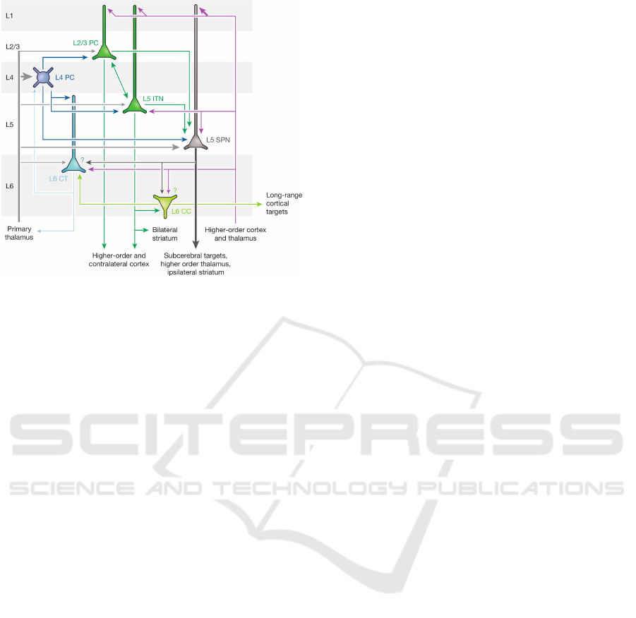
Figure 1: Canonical connectivity of cortical principal cells.

Reprinted with permission from (Harris and Mrsic-Flogel,

2013). PC: principal cell, ITN: intratelencephalic neuron,

SPN: subcerebral projection neuron, CT: corticothalamic

neuron, CC: corticocortical neuron. Line thickness repre-

sents the strength of a pathway, question marks indicate

connections that appear likely but have not yet been directly

shown.

wland et al., 2016), it can be demonstrated that their

behavior can also be interpreted as just one instance of

a more general information processing scheme (Ker-

dels and Peters, 2015; Kerdels, 2016). Here we ex-

tend this idea by generalizing and augmenting the pre-

vious grid cell model into an autoassociative memory

model describing the core function of a cortical mini-

column.

The next section revisits the grid cell model

(GCM) upon which the proposed autoassociative me-

mory model will be built. At its core the GCM is

based on the recursive growing neural gas (RGNG)

algorithm, which will also be a central component of

the new model. Section 3 introduces a ﬁrst set of

changes to the original GCM on the individual neu-

ron level that improve the long-term stability of lear-

ned representations, and allow the differentiation be-

tween processes occurring in the proximal and distal

sections of the neuron’s dendritic tree. In section 4

these changes are then integrated into a full autoasso-

ciative memory model, which consists of two distinct

groups of neurons that interact reciprocally. Section 5

presents preliminary results of early simulations that

support the basic assumptions of the presented model.

Finally, section 6 discusses the prospects of the propo-

sed perspective on cortical minicolumns and outlines

our future research agenda in that regard.

2 RGNG-BASED GRID CELL

MODEL

Grid cells are neurons in the entorhinal cortex of the

mammalian brain whose individual activity correlates

strongly with periodic patterns of physical locations

in the animal’s environment (Fyhn et al., 2004; Haf-

ting et al., 2005; Rowland et al., 2016). This property

of grid cells makes them particularly suitable for ex-

perimental investigation and provides a rare view into

the behavior of cortical neurons in a higher-order part

of the brain. The most prevalent view on grid cells

so far interprets their behavior as part of a specialized

system for navigation and orientation (Rowland et al.,

2016). However, from a more general perspective the

activity of grid cells can also be interpreted in terms

of a domain-independent, general information proces-

sing scheme as shown by the RGNG-based GCM of

Kerdels and Peters (Kerdels and Peters, 2015; Ker-

dels, 2016). The main structure of this model can be

summarized as follows: Each neuron is viewed as part

of a local group of neurons that share the same set of

inputs. Within this group the neurons compete against

each other to maximize their activity while trying to

inhibit their peers. In order to do so, each neuron tries

to learn a representation of its entire input space by

means of competitive Hebbian learning. In this pro-

cess the neuron learns to recognize a limited number

of prototypical input patterns that optimally originate

from maximally diverse regions of the input space.

This learned set of input pattern prototypes then con-

stitutes the sparse, pointwise input space representa-

tion of the neuron. On the neuron group level the

competition among the neurons forces the individual,

sparse input space representations to be pairwise dis-

tinct from one another such that the neuron group as

a whole learns a joint input space representation that

enables the neuron group to work as a sparse distri-

buted memory (Kanerva, 1988).

The GCM uses the recursive growing neural gas

algorithm (RGNG) to simultaneously describe both

the learning of input pattern prototypes on the level

of individual neurons as well as the competition bet-

ween neurons on the neuron group level. In contrast

to the common notion of modeling neurons as sim-

ple integrate and ﬁre units, the RGNG-based GCM

assumes that the complex dendritic tree of neurons

possesses more computational capabilities. More spe-

ciﬁcally, it assumes that individual subsections of a

neuron’s dendritic tree can learn to independently re-

cognize different input patterns. Recent direct obser-

vations of dendritic activity in cortical neurons sug-

gest that this assumption appears biologically plausi-

ble (Jia et al., 2010; Chen et al., 2013). In the model

A Grid Cell Inspired Model of Cortical Column Function

205

this intra-dendritic learning process is described by a

single growing neural gas per neuron, i.e., it is assu-

med that some form of competitive Hebbian learning

takes place within the dendritic tree. Similarly, it is

assumed that the competition between neurons on the

neuron group level is Hebbian in nature as well, and is

therefore modeled by analogous GNG dynamics. For

a full formal description and an in-depth characteri-

zation of the RGNG-based GCM we refer to (Kerdels

and Peters, 2016; Kerdels, 2016). In the following

section we focus on describing our modiﬁcations to

the original RGNG-based GCM.

3 EXTENDED NEURON MODEL

Although the neuron model outlined in the previous

section was conceived to describe the activity of en-

torhinal grid cells, it can already be understood as a

general computational model of certain cortical neu-

rons, i.e., L2/3 PC and L5 ITN in ﬁgure 1. However, to

function as part of our cortical column model we mo-

diﬁed the existing GCM with respect to a number of

aspects:

3.1 Ensemble Activity

In response to an input ξ the GCM returns an en-

semble activity vector a where each entry of a cor-

responds to the activity of a single neuron. Given a

neuron group of N neurons, the ensemble activity a

is calculated as follows: For each neuron n ∈ N the

two prototypical input patterns s

and s

that are clo-

sest to input ξ are determined among all prototypical

input patterns I

learned by the dendritic tree of neu-

ron n, i.e.,

:= argmin

v∈I

kv − ξk

:= argmin

v∈I

\{s

}

kv − ξk

The ensemble activity a := (a

,...,a

N−1

) of the

group of neurons is then given by

:= 1 −

− ξk

, i ∈ {0,.. .,N − 1}, (1)

followed by a softmax operation on a. Thus, the acti-

vity of each neuron is determined by the relative dis-

tances between the current input and the two best ma-

tching prototypical input patterns. If the input is about

equally distant to both prototypical input patterns the

activity is close to zero, and if the input is much clo-

ser to the best pattern than the second best pattern the

activity approaches one. The competition among the

neurons on the group level ensures that for any given

input only a small, but highly speciﬁc (Kerdels and

Peters, 2017) subset of neurons will exhibit a high

activation resulting in a sparse, distributed encoding

of the particular input.

Compared to the original GCM (Kerdels and Pe-

ters, 2016; Kerdels, 2016) we modiﬁed the activation

function (Eq. 1) to allow for a smoother response to

inputs that are further away from the best matching

unit s

than the distance between s

and s

, and we

normalized the ensemble output using the softmax

operation.

3.2 Learning Rate Adaptation

The original GCM uses ﬁxed learning rates ε

and ε

which require to ﬁnd a tradeoff between learning ra-

tes that are high enough to allow for a reliable adapta-

tion and alignment of initially random prototypes and

learning rates that are low enough to ensure a relati-

vely stable long-term representation of the respective

input space. We modiﬁed the original GCM in that re-

gard by introducing three learning phases that shape

the learning rates used by the GCM. During the initial

learning phase both ε

and ε

are kept at their initial

values (e.g., ε

= ε

= 0.01). The duration t

(measu-

red in # of inputs) of this ﬁrst phase depends on the

maximum number of prototypes M and the interval λ

with which new prototypes are added to the model

i.e., t

= 2Mλ. This duration ensures that the RGNG

underlying the GCM has enough time to grow to its

maximum size and to ﬁnd an initial alignment of its

prototypes. The second learning phase is a short tran-

sitional phase with a duration t

= Mλ in which both

learning rates ε

and ε

are reduced by one order of

magnitude to allow the initial alignment to settle in

a more stable conﬁguration. Up to this point the pro-

totypes learned by the individual neurons of the model

are likely to be similar as primary learning rate ε

and

secondary learning rate ε

are equal so far

. Begin-

ning with the last learning phase, which is open-ended

in its duration, only the secondary learning rate ε

reduced once more by two orders of magnitude. This

asymmetric reduction of ε

initiates a differentiation

process among the individual neurons that allows the

prototypes of each neuron to settle on distinct locati-

ons of the input space.

Both M and λ are parameters of the RGNG used by the

original GCM.

See (Kerdels, 2016) for details on how primary and se-

condary learning rates relate within an RGNG.

IJCCI 2018 - 10th International Joint Conference on Computational Intelligence

206

3.3 Handling of Repetitive Inputs

Since the GCM is a continuously learning model it

has to be able to cope with repetitive inputs in such

a way that its learned representation is not distorted

if it is exposed to a single repeated input. Without

adaptation a repeated input would correspond to an

artiﬁcial increase in learning rate. To handle such a

situation we adjust the learning rates ε

and ε

by an

attenuation factor ζ:

ζ = 0.1

|/10

with |s

| the number of successive times prototype s

was the best matching unit. The attenuation factor ζ

is applied when |s

| > 1.

3.4 Integration of Feedback Input

In order to use the GCM as part of our cortical co-

lumn model, we modiﬁed the existing GCM to allow

the integration of feedback connections. In the cor-

tex such feedback connections originate from higher-

order regions (violet arrows in Fig. 1) and predomi-

nantly terminate in layer 1 on the distal dendrites of

layer 2/ 3 and layer 5 neurons. To integrate these feed-

back connections into the model we added a secon-

dary GNG to the description of each neuron. With this

extension the dendritic tree of each neuron is now mo-

deled by two GNGs: a primary GNG that represents

the proximal dendrites that process the main inputs

to the neuron, and a secondary GNG that represents

the distal dendrites that process feedback inputs. Both

GNGs can independently elicit the neuron to become

active when either GNG receives a matching input.

If both GNGs receive inputs simultaneously, the out-

put o

of the primary GNG (determined by the ratio

shown in Eq. 1) is modulated by the output o

of the

secondary GNG depending on the agreement between

outputs o

and o

∗

1 + e

−

(

−φ

)(

1+γ

(

1−|o

−o

))

with parameter γ determining the strength of the mo-

dulation and parameter φ determining at which acti-

vity level (Eq. 1) of o

the output is increased or de-

creased, respectively. Typical values are, e.g., γ = 10

and φ = 0.5.

A second important relation between the primary

and the secondary GNG concerns learning of new

prototypical input patterns. The secondary GNG can

only learn when the primary GNG has received a ma-

tching input that resulted in an activation of the neu-

ron, i.e., the learning rates ε

and ε

of the secondary

GNG are scaled by the output of the primary GNG in

response to a current main input to the neuron:

∗

:= ε

∗

:= ε

or by zero if there is no main input present. As a con-

sequence, the secondary GNG learns to represent only

those parts of the feedback input space that correlate

with regions of the main input space that are directly

represented by the prototypical input patterns of the

primary GNG. This way, the secondary GNG learns to

respond only to those feedback signals that regularly

co-occur with those main input patterns that were le-

arned by the primary GNG. One possible neurobiolo-

gical mechanism that could establish such a relation

between proximal and distal dendrites is the back-

propagation of action potentials (Stuart et al., 1997;

Waters et al., 2005).

Together, the primary and secondary GNG allow

a modeled neuron to learn a representation of its main

input space while selectively associating feedback in-

formation that may help to disambiguate noisy or dis-

torted main input or substitute such input if it is mis-

sing.

4 CORTICAL COLUMN MODEL

So far the extended neuron model describes a single

group of neurons that is able to learn a sparse, dis-

tributed representation of its input space and is able

to integrate additional feedback input. As such, the

group acts as a local, input-driven transformation that

maps input signals to output signals without maintai-

ning an active state, i.e., if no input is present, no

output will be generated. However, if two groups

share the same main input space but also receive the

group activity of each other as an additional input sig-

nal, both groups would be able to maintain a stable

active state even when the main input signal vanis-

hes. Instead of being stateless input-output transfor-

mations the two groups would form an active autoas-

sociative memory cell (AMC) (Kanerva, 1988; Ka-

nerva, 1992). Given the canonical connectivity of

cortical principal cells shown in ﬁgure 1 we argue

that L2/3 PC and L5 ITN constitute such a pair of reci-

procally connected neuron groups forming an AMC.

Both groups share a main input space via connecti-

ons from the primary thalamus and local L4 PC, while

they also both receive feedback input at their distal

dendrites in layer 1 from higher-order cortex and the

thalamus

These feedback connections motivated the extension

described in section 3.4.

A Grid Cell Inspired Model of Cortical Column Function

207

The other neuron groups shown in ﬁgure 1 can be

interpreted as providing support for the AMC: The

outputs of both L2/3 PC and L5 ITN connect locally to

L5 SPN, which projects to subcerebral targets, e.g.,

motor centres, and non-locally to higher-order parts

of the cortex. The output of the lower group L5 ITN

makes an additional local connection to L6 CC, which

projects to long-range cortical targets, but also locally

to L6 CT, which in turn connects back to L4 PC and the

primary thalamus.

We propose that the described neural structure

constitutes a single cortical minicolumn. At its core

the minicolumn hosts a single autoassociative me-

mory cell (L2/3 PC / L5 ITN) that is supported by neu-

rons regulating its activity (L4 PC), its input (L4 PC /

L6 CT) and its output (L5 SPN / L6 CC).

A key property of the described AMC is its ability

to feed its output back into itself via the reciprocal

connections between the two neuron groups ( L2/3 PC

/ L5 ITN). This local feedback loop does not only allow

the AMC to stay active when the main input vanis-

hes. It also enables a form of attractor dynamics (Ka-

nerva, 1988; Kanerva, 1992) where an initial, poten-

tially noisy or ambiguous input pattern can be itera-

tively reﬁned to approach one of the stable, prototy-

pical input patterns learned by the AMC. In addition,

this iterative process can be supported or modulated

by the feedback input integrated via the distal den-

drites of both neuron groups. On a cortex-wide level

these attractor dynamics might play an important role

to dynamically bind subsets of cortical minicolumns

into joint, temporarily stable attractor states.

5 PRELIMINARY RESULTS

As a ﬁrst step towards implementing the cortical co-

lumn model outlined in the previous section we simu-

lated a single AMC consisting of two neuron groups

a and b, which correspond to the two neuron groups

L2/3 PC and L5 ITN of ﬁgure 1. Each neuron group was

modeled by the extended GCM described in section 3

containing 25 neurons with 16 dendritic prototypes

each. Further parameters are given in table 1. As in-

put both groups received samples from the MNIST

database of handwritten digits (Lecun et al., 1998) re-

duced to a resolution of 16 × 16 pixels concatenated

with the current ensemble activity of the other group.

Each MNIST input was repeated 10× in a row combi-

ned in each case with the updated ensemble activity of

the respective other neuron group allowing for the co-

occurrence of the original input with the other group’s

reaction to that input. In total, the simulated AMC

was presented with 20 million inputs corresponding

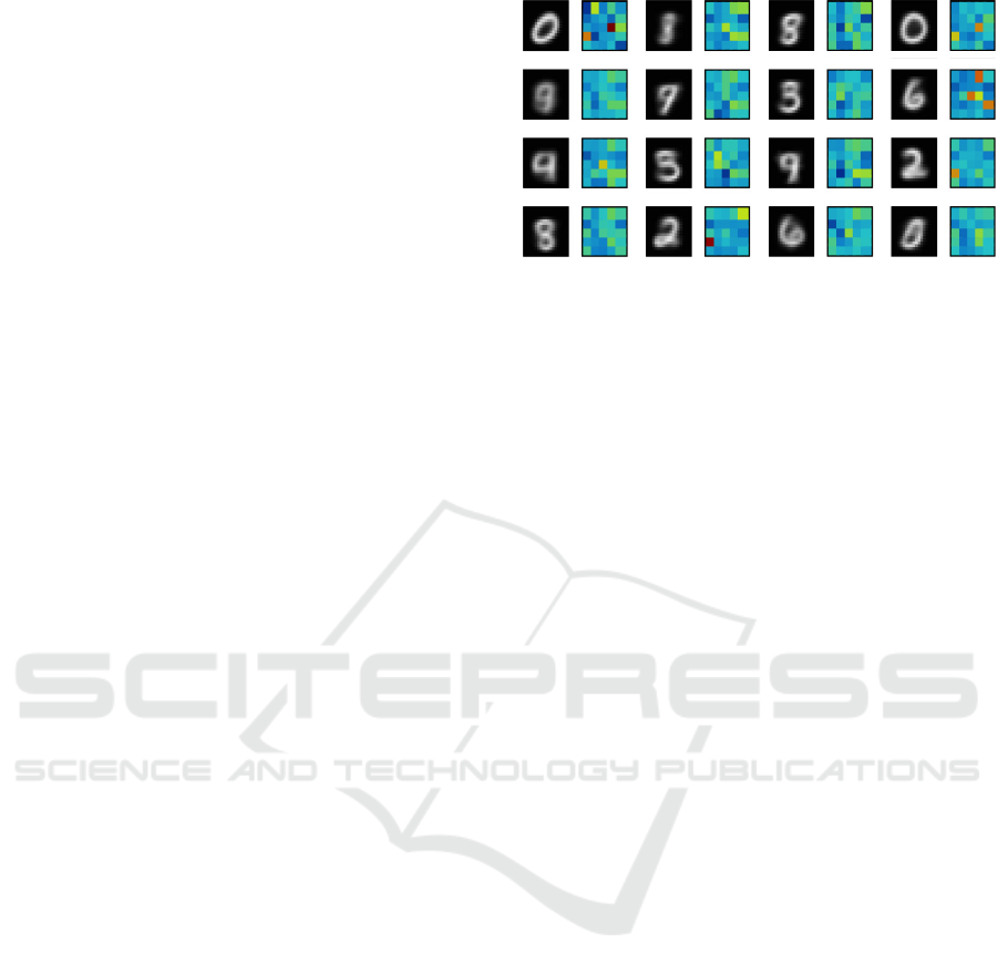
Figure 2: Sixteen prototypes learned by a single neuron of

neuron group a. Each prototype consists of a 16 × 16 re-

presentation corresponding to the MNIST part of the input

(shown in gray) and a 5×5 representation corresponding to

the group b ensemble activation part of the input (visuali-

zed as color gradient from blue (low activation) to red (high

activation).

to about 33 full presentations of the MNIST training

data set to the system.

Figure 2 shows the 16 dendritic prototypes lear-

ned by a single neuron of group a after a total of

20 million inputs. Like the input patterns the pro-

totypes consist of two parts: a 16 × 16 representa-

tion corresponding to the MNIST portion of the in-

put and a 5 × 5 representation corresponding to the

ensemble activation of neuron group b co-occurring

with the particular MNIST inputs. The MNIST part

of the prototypes indicate that the neuron is, as ex-

pected, learning a sparse, pointwise representation of

its entire input space. While some prototypes exhi-

bit clear and distinct shapes that indicate that these

prototypes have already settled at stable locations in

input space, a few prototypes have less distinct shapes

indicating that these prototypes have not yet reached

such stable locations. One important aspect to note is

that this neuron will exhibit a high activity for any of

the learned input patterns. As a consequence, looking

just at the activity of this individual neuron it is not

possible to tell whether the input was a, e.g., “0” or

“2” or any of the other patterns represented by one of

the neuron’s prototypes.

A disambiguation of the input becomes only pos-

sible when observing the ensemble activity of an en-

tire neuron group, i.e., the representation of the input

is distributed across the entire group. No individual

neuron encodes for just a single input. Such ensem-

ble activities are captured by the ensemble part of the

prototypes and show, in this case, the average ensem-

ble activity of group b in response to the respective

MNIST input captured by the MNIST part of the pro-

totypes. The ensemble activities of group b shown in

ﬁgure 2 show that each input pattern evokes a distinct

pattern of ensemble activity allowing to disambiguate

the different input patterns. In case of already stable

IJCCI 2018 - 10th International Joint Conference on Computational Intelligence

208

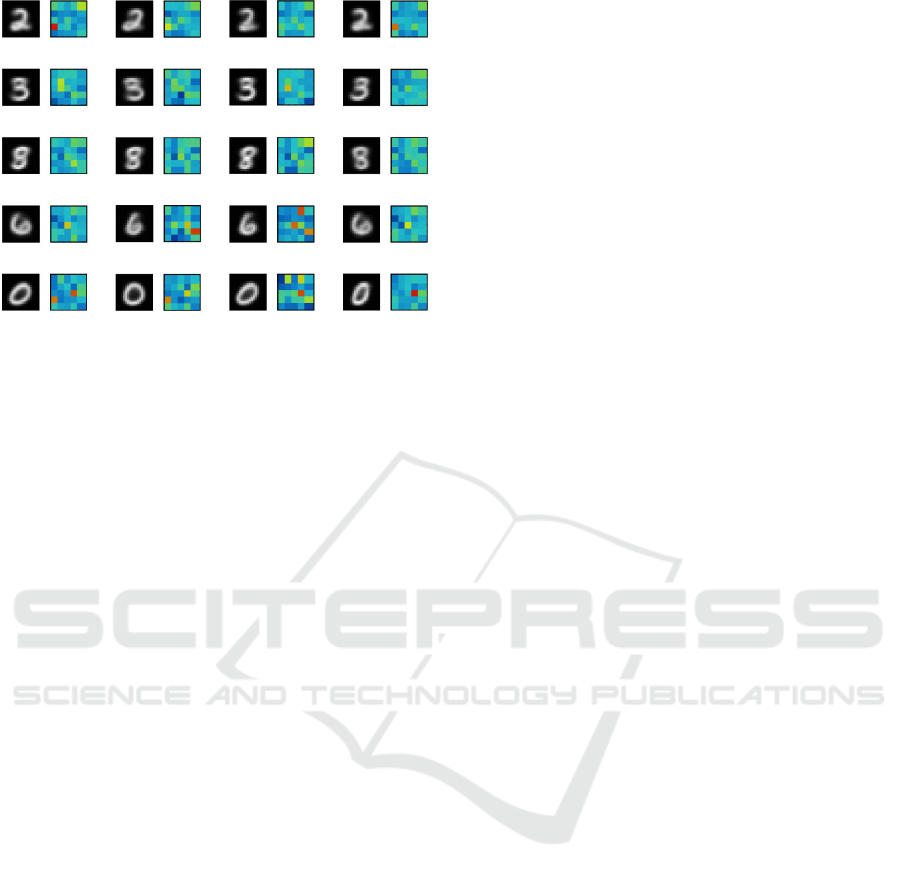
Figure 3: Twenty examples of learned prototypes from dif-

ferent neurons of group a that represent numbers of similar

shape. Visualization as in Fig. 2.

prototypes it can also be seen, that the ensemble acti-

vity tends to be sparse with only a few neurons exhi-

biting a strong activation in response to a particular

input.

One interesting question regarding such a sparse,

distributed representation is the degree of variation in

this ensemble code if very similar inputs are proces-

sed. Figure 3 shows twenty examples of dendritic pro-

totypes from different neurons of group a that repre-

sent numbers of similar shape. The captured ensem-

ble activities of group b indicate that the similarity of

activation patterns appears to match well with the si-

milarity of the corresponding MNIST patterns. Even

in cases with an overall low activation like the respon-

ses to the number “8” (third row), the corresponding

ensemble codes appear similar.

These ﬁrst tentative results indicate, that the pro-

posed model appears to be able to learn a sparse, dis-

tributed representation of its main input space (here

the MNIST set), while simultaneously learning the

ensemble codes of an accompanying group of neu-

rons that operates on the same input space.

6 CONCLUSION

The cortical column model outlined in this paper is

still in a very early stage. Yet, it combines multiple,

novel ideas that will guide our future research. First,

the RGNG-based, unsupervised learning of a sparse,

distributed input space representation utilizes a clas-

sic approach of prototype-based learning in a novel

way. Instead of establishing a one-to-one relation be-

tween a learned representation (prototype) and a cor-

responding region of input space, it learns an ensem-

ble code that utilizes the response of multiple neurons

(sets of prototypes) to a given input. The presented

preliminary results indicate that learning such an en-

semble code appears feasible. Our future research in

this regard will focus on improving our understanding

of the resulting ensemble code, as well as improving

the RGNG algorithm in terms of learning speed and

robustness w.r.t. a continuous learning regime.

Second, the idea of reciprocally connecting two

neuron groups that process a shared input space ena-

bles the creation of an autoassociative memory cell

(AMC) that is able to maintain an active state even in

the absence of any input. In addition, such an AMC

may exhibit some form of attractor dynamics where

the activities of the two, reciprocally connected neu-

ron groups self-stabilize. A precondition for such an

AMC is the groups’ ability to learn the ensemble code

of the respective other group. The presented prelimi-

nary results indicate that this is possible. Our future

research will focus on understanding the characteris-

tics of the dynamics of such an AMC, e.g., in response

to various kinds of input disturbances.

Third, the outlined cortical column model sug-

gests that the cortex may consist of a network of

autoassociative memory cells that inﬂuence each ot-

her via feedback as well as feedforward connections

while trying to achieve locally stable attractor states.

In addition, further cortical circuitry may modulate

the activity of individual cortical columns to facilitate

competition among cortical columns or groups of cor-

tical columns on a more global level, which may then

lead to the emergence of stable, global attractor states

that are able to temporarily bind together sets of corti-

cal columns. In this context our research is still in its

infancy and will focus on implementing a ﬁrst version

of a full cortical column model that can then be tested

in small hierarchical network conﬁgurations, e.g., to

process more complex visual input.

REFERENCES

Buxhoeveden, D. P. and Casanova, M. F. (2002). The

minicolumn hypothesis in neuroscience. Brain,

125(5):935–951.

Chen, T.-W., Wardill, T. J., Sun, Y., Pulver, S. R., Rennin-

ger, S. L., Baohan, A., Schreiter, E. R., Kerr, R. A.,

Orger, M. B., Jayaraman, V., Looger, L. L., Svoboda,

K., and Kim, D. S. (2013). Ultrasensitive ﬂuores-

cent proteins for imaging neuronal activity. Nature,

499(7458):295–300.

Fyhn, M., Molden, S., Witter, M. P., Moser, E. I., and Mo-

ser, M.-B. (2004). Spatial representation in the entor-

hinal cortex. Science, 305(5688):1258–1264.

Hafting, T., Fyhn, M., Molden, S., Moser, M.-B., and Mo-

ser, E. I. (2005). Microstructure of a spatial map in

the entorhinal cortex. Nature, 436(7052):801–806.

A Grid Cell Inspired Model of Cortical Column Function

209

Harris, K. D. and Mrsic-Flogel, T. D. (2013). Cortical con-

nectivity and sensory coding. Nature, 503:51.

Hashmi, A. G. and Lipasti, M. H. (2009). Cortical columns:

Building blocks for intelligent systems. In 2009 IEEE

Symposium on Computational Intelligence for Multi-

media Signal and Vision Processing, pages 21–28.

Hawkins, J., Ahmad, S., and Cui, Y. (2017). Why does

the neocortex have columns, a theory of learning the

structure of the world. bioRxiv.

Horton, J. C. and Adams, D. L. (2005). The cortical co-

lumn: a structure without a function. Philosophical

Transactions of the Royal Society of London B: Biolo-

gical Sciences, 360(1456):837–862.

Jia, H., Rochefort, N. L., Chen, X., and Konnerth, A.

(2010). Dendritic organization of sensory input to cor-

tical neurons in vivo. Nature, 464(7293):1307–1312.

Kanerva, P. (1988). Sparse Distributed Memory. MIT Press,

Cambridge, MA, USA.

Kanerva, P. (1992). Sparse distributed memory and related

models [microform] / Pentti Kanerva. Research In-

stitute for Advanced Computer Science, NASA Ames

Research Center.

Kerdels, J. (2016). A Computational Model of Grid Cells

based on a Recursive Growing Neural Gas. PhD the-

sis, FernUniversit

at in Hagen.

Kerdels, J. and Peters, G. (2015). A new view on grid cells

beyond the cognitive map hypothesis. In 8th Confe-

rence on Artiﬁcial General Intelligence (AGI 2015).

Kerdels, J. and Peters, G. (2016). Modelling the grid-like

encoding of visual space in primates. In Proceedings

of the 8th International Joint Conference on Compu-

tational Intelligence, IJCCI 2016, Volume 3: NCTA,

Porto, Portugal, November 9-11, 2016., pages 42–49.

Kerdels, J. and Peters, G. (2017). Entorhinal grid cells may

facilitate pattern separation in the hippocampus. In

Proceedings of the 9th International Joint Conference

on Computational Intelligence, IJCCI 2017, Funchal,

Madeira, Portugal, November 1-3, 2017., pages 141–

148.

Lecun, Y., Bottou, L., Bengio, Y., and Haffner, P. (1998).

Gradient-based learning applied to document recogni-

tion. Proceedings of the IEEE, 86(11):2278–2324.

Mountcastle, V. B. (1978). An organizing principle for ce-

rebral function: The unit model and the distributed

system. In Edelman, G. M. and Mountcastle, V. V.,

editors, The Mindful Brain, pages 7–50. MIT Press,

Cambridge, MA.

Mountcastle, V. B. (1997). The columnar organization of

the neocortex. Brain, 120(4):701–722.

Rinkus, G. J. (2017). A cortical sparse distributed coding

model linking mini- and macrocolumn-scale functio-

nality. ArXiv e-prints.

Rowland, D. C., Roudi, Y., Moser, M.-B., and Moser, E. I.

(2016). Ten years of grid cells. Annual Review of

Neuroscience, 39(1):19–40. PMID: 27023731.

Stuart, G., Spruston, N., Sakmann, B., and Husser, M.

(1997). Action potential initiation and backpropaga-

tion in neurons of the mammalian cns. Trends in Neu-

rosciences, 20(3):125 – 131.

Waters, J., Schaefer, A., and Sakmann, B. (2005). Back-

propagating action potentials in neurones: measure-

ment, mechanisms and potential functions. Progress

in Biophysics and Molecular Biology, 87(1):145 –

170. Biophysics of Excitable Tissues.

APPENDIX

Parameterization

The neuron groups modeled by the extended GCM

described in section 3 use an underlying, two-layered

RGNG. Each layer of an RGNG requires its own set

of parameters. In this case we use the sets of parame-

ters θ

and θ

, respectively. Parameter set θ

controls

the inter-neuron level of the GCM while parameter

set θ

controls the intra-neuron level. Table 1 sum-

marizes the parameter values used for the simulation

runs presented in this paper. For a detailed charac-

terization of these parameters we refer to (Kerdels,

2016).

Table 1: Parameters of the RGNG-based, extended GCM

used for the preliminary results presented in section 5. For

a detailed characterization of these parameters we refer to

the appendix and (Kerdels, 2016).

= 0.04 ε

= 0.01

= 0.04 ε

= 0.01

= 0.01 ε

= 0.01

λ = 1000 λ = 1000

τ = 100 τ = 100

α = 0.5 α = 0.5

β = 0.0005 β = 0.0005

M = 25 M = 16

IJCCI 2018 - 10th International Joint Conference on Computational Intelligence

210