
Automatic Detection of Subassemblies for Disassembly Sequence
Planning
Yongjing Wang
1
, Feiying Lan
1
, Duc Truong Pham
1
, Jiayi Liu
1,2
, Jun Huang
1
, Chunqian Ji
1
,
Shizhong Su
1
, Wenjun Xu
2,3
, Quan Liu
2,4
and Zude Zhou
4,5
1
Autonomous Remanfuatcuring Laboratory, Department of Mechanical Engineering,
The University of Birmingham, Edgbaston, Birmingham, B15 2TT, U.K.
2
School of Information Engineering, Wuhan University of Technology, Wuhan, 430070, China
3
Hubei Key Laboratory of Broadband Wireless Communication and Sensor Networks,
Wuhan University of Technology, Wuhan, 430070, China
4
Key Laboratory of Fibre Optic Sensing Technology and Information Processing (Ministry of Education),
Wuhan University of Technology, Wuhan, 430070, China
5
School of Mechanical and Electronic Engineering,
Wuhan University of Technology, Wuhan, 430070, China
Keywords: Remanufacturing, Disassembly Planning, Dismantling, Robotic Disassembly.
Abstract: Disassembly, the first process in remanufacturing, is labour-intensive due to the conditions of end-of-life
products returned for remanufacture. Robotic disassembly is an attractive alternative to manual disassembly
but robotic systems cannot plan disassembly sequences automatically and manual planning is still required.
Several planning methods have been proposed to take away removable components sequentially. However,
those methods do not work when it is required to break an assembly into subassemblies. This paper proposes
a method for automatic detection of subassemblies. The approach starts with using an assembly matrix and
simple logic gates to generate a contact matrix and a relation matrix. The paper details new algorithms used
to detect subassemblies through manipulating the two matrices.
1 INTRODUCTION
Remanufacturing is "the rebuilding of a product to
specifications of the original manufactured product
using a combination of reused, repaired and new
parts" (Johnson and McCarthy, 2014). One
important feature distinguishing remanufacturing
from conventional manufacturing is disassembly.
Due to the variability in the condition of the returned
products, disassembly tends to be manually carried
out. It is labour intensive, given the complexity of
the operations involved.
Developments in automated disassembly
systems started in the mid-1990s with the robotic
disassembly of a PC (Kopacek and Kronreif, 1996),
followed by several successful attempts at
dismantling electrical devices and automotive
components (Barwood et al., 2015; Gil et al., 2007;
Vongbunyong and Chen, 2015). The reported
experiments were mostly product-orientated and
based on pre-programmed sequences. A key
advance from ‘automated’ disassembly to
‘autonomous’ disassembly would be that machines
plan disassembly sequences using the structure of
the product rather than following a pre-programmed
sequence. A popular approach is based on graphs (Li
et al., 2002; Torres et al. , 2003). Many algorithms
and rule-based methods have been used to calculate
disassembly sequences, for example, the Fuzzy
Reasoning Petri Net proposed by Zhao and Li (Zhao
and Li, 2010). However, the generation of a graph
relies on human understanding instead of machine
interpretation.
Smith et al. presented a tool consisting of five
matrices to represent an assembly and used several
rules to generate disassembly sequences (Smith and
Chen, 2009; Smith et al., 2012). Tao et al. also
modified the matrices to enable partial/parallel
94
Wang, Y., Lan, F., Pham, D., Liu, J., Huang, J., Ji, C., Su, S., Xu, W., Liu, Q. and Zhou, Z.
Automatic Detection of Subassemblies for Disassembly Sequence Planning.
DOI: 10.5220/0006906600940100
In Proceedings of the 15th International Conference on Informatics in Control, Automation and Robotics (ICINCO 2018) - Volume 1, pages 94-100
ISBN: 978-989-758-321-6
Copyright © 2018 by SCITEPRESS – Science and Technology Publications, Lda. All rights reserved
disassembly (Tao et al., 2017). However, this
optimisation-focused work did not reduce the
complexity of the mathematical representation of an
assembly in which distinguishing between fasteners
and general parts was needed although their
definitions were fuzzy and could cause confusion in
many cases. For example, it is not clear whether to
categorise objects in press-fit components as
fasteners or general parts. Another matrix-based
example can be found in the work of Jin et al. (Jin
et al., 2015; Jin et al., 2013), in which the
relationships between components were presented
using just a matrix. However, the matrix-based
methods tend to focus on sequential disassembly and
cannot work correctly when breaking an assembly
into subassemblies is required.
This paper presents a method that can detect
subassemblies automatically. Based on an analysis
of over 239 mechanical products by the authors’
team, breaking into subassemblies is a critical step
for some 23% of them (Ji et al. 2017), and cannot be
correctly dealt with using conventional methods.
Section 2 presents the definitions and derivations
of two matrices: contact and relation matrix, which
can represent the contact status of components. Such
information can be used to identify separable pairs,
pairs of components which can be broken to build
subassemblies (Section 3). A case study is given in
Section 4 to demonstrate the use of the approach.
2 CONTACT AND RELATION
MATRICES: FUNDAMENTAL
TOOLS
Jin et al. (Jin et al., 2015; Jin et al., 2013) demons-
trated a method to identify removable components
to generate feasible disassembly sequences using the
space interference matrix. The essence of the
approach is to find components that have freedom in
at least one direction, indicating that the components
are removable. A product can be disassembled after
multiple cycles of taking away removable
components step-by-step in a sequential way.
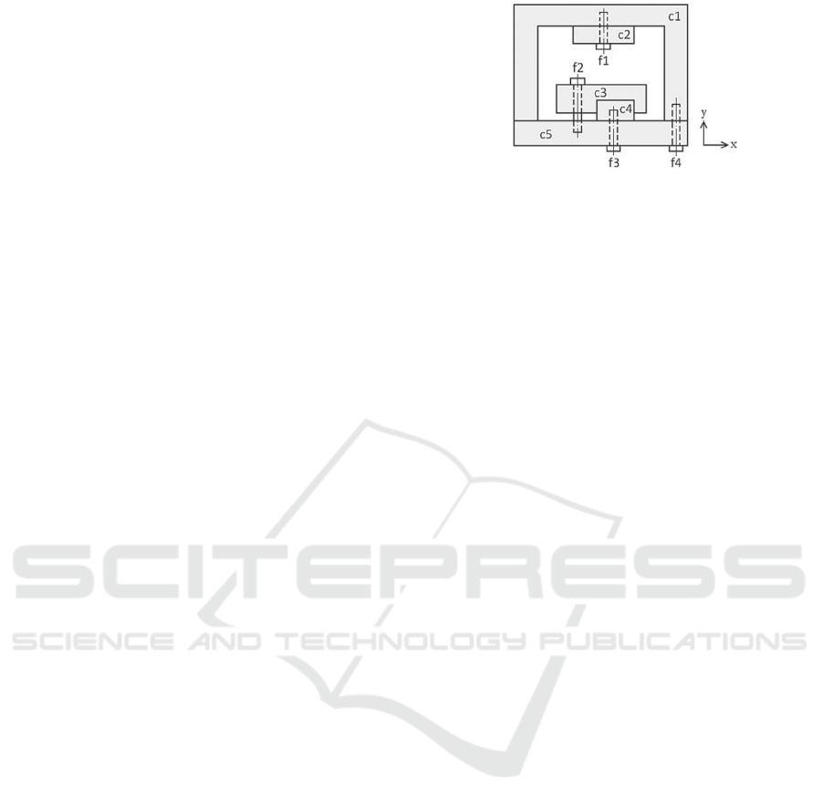
Figure 1: An example product.
If the method is adopted for the case in Figure 1
(Smith and Hung, 2015), however, after the removal
of
and
in the first step, no components can be
further disassembled, as shown in Figure 2. This is
a typical interlocking structure. An assembly cannot
be disassembled as no parts are removable until the
whole structure is broken into smaller
subassemblies.
The paper proposes the contact matrix
and relation matrix, as fundamental tools to
detect subassemblies. It can represent contact
conditions in an assembly in six directions
(X+, X-, Y+, Y-, Z+, Z-). Here, only four directions
(X+, X-, Y+, Y-) are needed for demonstrations in
two dimensions, as shown in Eq. 1.
In the matrix,
represents components in an
assembly.
.
,
.
,
.
, and
.
indicate
the contact status of the components in the
corresponding columns and rows by using two
states: 0 for no contact and 1 for contact. For
example, the assembly in Figure 1 can be
represented by the contact matrix in Eq. 2.
.
.
.
.
is 0001 because
is a
contact in Y- direction for
.
can be removed
from
in Y+ direction. Similarly,
.
.
.
.
is 0010 because
a contact
in Y+ direction for
.
can be removed from
in Y- direction. It is worth noting that symmetry may
not be observed in
.
.
.
.
and
.
.
.
.
due to requirements of
proper disassembly operations. For example,
.
.
.
.
is 1110 and
.
.
.
.
is 1111, because removing
from
is a proper operation but the reverse is not.
The relation matrix describes the general contact
status of components, derived from contact matrix
(Figure 3). The two matrices could be the keys for a
machine to understand subassemblies.
Automatic Detection of Subassemblies for Disassembly Sequence Planning
95
Figure 2: Sequential disassembly method proposed by Jin et al. (Jin et al., 2015; Jin et al., 2013).
…
=
⋮
.
.
.
.
⋯
.
.
.
.
⋮⋱⋮
.
.
.
.
⋯
.
.
.
.
(1)
C=
0000 0001 0000 0000 0001 1111 0000 0000 1111
0010 0000 0000 0000 0000 1111 0000 0000 0000
0000 0000 0000 1101 0000 0000 1111 0000 0000
0000 0000 1110 0000 0001 0000 0000 1111 0000
0010 0000 0000 0010 0000 0000 1111 1111 1111
1110 1110 0000 0000 0000 0000 0000 0000 0000
0000 0000 1101 0000 1101 0000 0000 0000 0000
0000 0000 0000 1110 1110 0000 0000 0000 0000
1110 0000 0000 0000 1110 0000 0000 0000 0000
(2)
Figure 3: Derivation of a relation matrix from a contact matrix.
3 SEPARABILITY CHECK
3.1 Definition of Separability
The separability of an assembly indicates whether it
can be broken into subassemblies. The separability of
an assembly is determined by whether it contains
‘separable pairs’, pairs of contacting components that
can be separated without affecting other contacting
components. For example, the assembly in Figure 4a
has three components: A1, B1 and C1, and two pairs
of contacting components: A1-B1 and B1-C1. If a
contact between a pair can be represented as a line,
ICINCO 2018 - 15th International Conference on Informatics in Control, Automation and Robotics
96
then the physical model in Figure 4a can be simplified
to Figure 4b, which can also be represented by its
relation matrix (R1), as shown in Figure 4c. Both
pairs, A1-B1 and B1-C1, are separable, as the
separation of either pair would not affect the other.
Figure 4: An example of a product comprising separable
pairs.
However, in a similar model shown in Figure 5,
the result would be different. None of the three pairs,
A2-B2, B2-C2 and A2-C2, are separable, as the
separation of a pair could affect other pairs. For
example, the separation of A2-B2 inevitably causes
the detachment of A2 from C2. Comparing Figure 4b
to Figure 5b, it is obvious that there is only one path
between A1 and B1 (A1-B1) in Figure 4b, but there
are two paths between A2 and B2 (A2-B2, and A2-
C2-B2) in Figure 5b. When there is only one path, the
interaction between the two components is not
coupled with those with other components. A
sufficient condition for a pair to be separable is that
there is only one path between two components in a
pair, as in the pairs A1-B1 and B1-C1 in Figure 4b.
Figure 5: An example of a product comprising inseparable
pairs.
3.2 Separable Pairs Search Process
Separable pairs can be searched for using vectors,
namely node vectors, to represent components, as
shown in Eq. 3, so that the links connected to a node
can be calculated by multiplying the relation matrix
R1 with its note vector (Eq. 4 to 6).
1=
1
0
0
,1=
0
1
0
,1=
0
0
1
(3)
R1.
1=
010
101
010
∙
1
0
0
=
0
1
0
=1,
R1.1=
010
101
010
∙
0
1
0
=
1
0
1
=1+1,
R1.C1=
010
101
010
∙
0
0
1
=
0
1
0
=1
(4)
(5)
(6)
The method can be used to identify adjacent
components. Also, a path between two nodes can be
found by recursively multiplying the relation matrix
by a node vector and its adjacent node vectors until a
destination is reached. Figure 6 shows the process of
searching for separable pairs using a relation matrix.
Figure 6: Separable pairs search process.
The first step is to search for adjacent pairs, two
components in contact, which can be identified using
Eq. 3 to 6.
The second step is to identify the pair in which
there is only one route between the two components,
a sufficient condition for a pair to be separable, as
discussed earlier. We propose using a recursive
strategy using the pseudo code in Algorithm 1.
Automatic Detection of Subassemblies for Disassembly Sequence Planning
97
Algorithm 1: Generate single-path pair list from adjacent
pair list.
Main function:
Input: adjacent pair list (APL)
Output: Single-path list (SPL)
1 For every pair {X, Y} Є APL
2 counter = 0
3 searchPath(X,Y) ;
4 If counter = 1
5 add {X, Y} to SPL;
6 End if
7 End for
searchPath(X,Y)
8 Label X as discovered
9 For every component k adjacent to X
10 If k is not labelled as discovered
11 If k = Y
12 counter++;
13 If counter >=2
14 break;
15 End if
16 Else
17 Recursively call searchPath(k,Y)
18 End if
19 End if
19 Return counter
20 End for
After all single-path pairs are identified,
their corresponding elements in the contact
matrix should be checked. If the elements are
not 1111 (
.
.
.
.
≠1111 and
.
.
.
.
≠1111), it indicates that one
component has freedom on at least one direction in
relation to the other, and thus the pair is separable.
Details are explained using the discussed example in
Figure 1.
After the removal of
and
, the node-line
model of the assembly and its relation matrix are
presented in Figure 7 and Eq. 7. By using Eqs.3 and
4, eight adjacent pairs can be identified: C1-C2, C1-
C4, C2-C3, C2-f1, C3-C4, C4-C5, C5-f1 and C5-f2.
Figure 7: Model of the assembly after the removal of f3 and
f4.
R=
0101010
1010000
0101000
1010100
00010
11
1000101
0000110
(7)
Algorithm 1 is used to calculate the number of
routes between two components in a pair, starting
from the first pair C1-C2. The result indicates that the
pair is not separable, as there are two routes from C1
to C2 (C1→C2 and C1→f1→C2), as depicted in
Figure 8. For the next member on the adjacent pair
list, C1-C5, only one route is found, and thus the pair
is added to single-path list. The calculation continues
for all pairs on the adjacent pair list, and C1-C5 is the
only single-path pair. As C1 and C5 have freedom in
3 directions, the pair is a separable pair.
Figure 8: An example of searching for single-path pairs.
It indicates that the separation of C1 and C5 would
result in two subassemblies: C1-C2-f1 and C3-C4-
C5-f2. Then, f2 and f1 become removable and
disassembly iterations could carry on using sequential
disassembly planning methods.
4 CASE STUDY
This section discusses a case study of the disassembly
of a piston used in a 4-stroke engine, as shown in
Figure 9.
ICINCO 2018 - 15th International Conference on Informatics in Control, Automation and Robotics
98
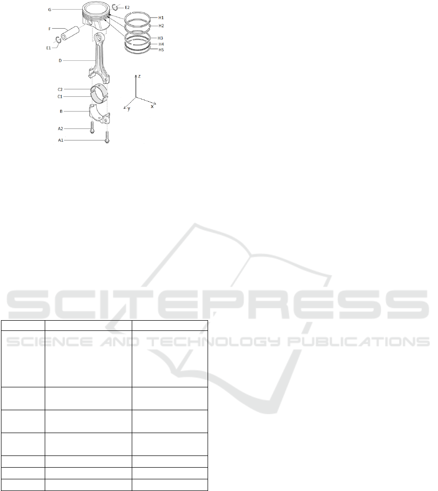
Figure 9: Parts in a piston.
If the conventional sequential disassembly
method (G. Jin et al., 2015; G. Q. Jin et al., 2013) is
adopted, the sequential disassembly plan as shown in
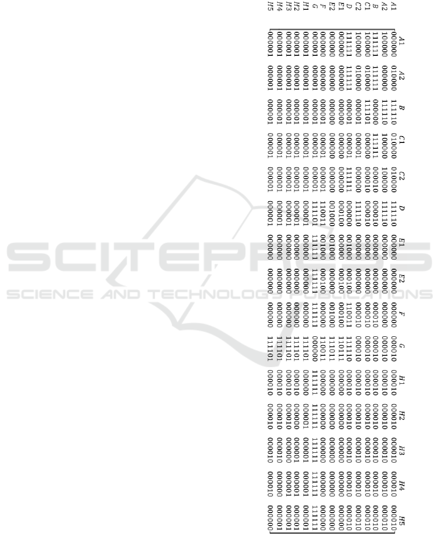
table 1 is obtained using the space interference matrix
(Appendix). It can be seen that no removable parts are
identified at iteration 7, and parts B, C1-2 and D form
an interlocking structure. To continue disassembly,
the methods presented in Section 3 can be employed
to identify a separable pair to break the product into
subassemblies.
Table 1: Sequential disassembly plan generated using the
method by Jin et al.
Iteration Removable parts Remaining parts
1
A1-111110
A2-111110
E1-110111
E2-111011
H1-111101
B, C1-2, D, F, G,
H2-5
2
F -110011
H2 - 111101
B, C1-2, D, G,
H3-5
3
H3 - 111101 B, C1-2, D, G,
H4-5
4
H4 - 111101 B, C1-2, D, G,
H5
5 H5 - 111101 B, C1-2, D, G
6 G - 111101 B, C1-2, D
7 None B, C1-2, D
The contact matrix and related matrix of the
structure B-C1-C2-D are given in Eqs. 8 and 9. By
using Eq. 3 to 6, three adjacent pairs can be identified:
B-C1, B-D and C2-D. Algorithm 1 is used to calculate
the number of routes between two components in a
pair. The result indicates that all three pairs are single-
path pairs. However, only B-D is a separable pair as
C
12
and C
43
are 111111, indicating that either B-C1 or
C2-D has no freedom to separate. The separation of
B and D builds two subassemblies, B-C1 and C2-D,
and thus further disassembly operations can carry on.
C=
1 2
1
2
000000 111111
111101 000000
000000 000010
000000 000000
000000 000000
000001 000000
000000 111110
111111 000000
(8)
=
12
1
2
01
10
01
00
00
10
01
10
(9)
5 CONCLUSION
Machine understanding of the structure of an assembly
in three-dimensional space is required for autonomous
disassembly planning. Conventionally, because of the
complexity of spatial information, models tended to be
complex and normally not suitable for all structures, in
particular, those containing interlocking components.
As far as the authors are aware, no previous work has
been carried out relating to this issue.
This paper presents a method to break an
assembly into subassemblies when sequential
disassembly of components is not possible. The
method is designed to work for all subassemblies
containing interlocking components and its
effectiveness was demonstrated with a case study.
Future work could investigate combining the
proposed method with conventional disassembly
planning approaches. This would undoubtedly yield a
more capable disassembly planning system suitable
for adoption in autonomous remanufacturing.
ACKNOWLEDGEMENT
This research was supported by the EPSRC (Grant
No. EP/N018524/1) and the National Science
Foundation of China (Grant No. 51775399).
REFERENCES
Barwood, M., Li, J., Pringle, T., and Rahimifard, S. (2015).
Utilisation of reconfigurable recycling systems for
improved material recovery from e-waste. In Procedia
CIRP (Vol. 29, pp. 746–751). https://doi.org/10.1016/
j.procir.2015.02.071
Gil, P., Pomares, J., Puente, S. V. T., Diaz, C., Candelas, F.,
and Torres, F. (2007). Flexible multi-sensorial system
for automatic disassembly using cooperative robots.
International Journal of Computer Integrated
Manufacturing, 20(8), 757–772. https://doi.org/ 10.10
Automatic Detection of Subassemblies for Disassembly Sequence Planning
99
80/09511920601143169
Ji, C., Pham, D. T., Su, S., Huang, J., and Wang, Y. (2017).
AUTOREMAN – D.1.1 - List of generic disassembly
task categories, Technical Report, Autonomous Rema-
nufacturing Laboratory, the University of Birmingham.
Jin, G., Li, W., Wang, S., and Gao, S. (2015). A systematic
selective disassembly approach for Waste Electrical
and Electronic Equipment with case study on liquid
crystal display televisions. Proceedings of the
Institution of Mechanical Engineers, Part B: Journal of
Engineering Manufacture. https://doi.org/10.1177/09
54405415575476
Jin, G. Q., Li, W. D., and Xia, K. (2013). Disassembly
Matrix for Liquid Crystal Displays Televisions.
Procedia CIRP, 11, 357–362. https://doi.org/10.1016/
j.procir.2013.07.015
Johnson, M. R., and McCarthy, I. P. (2014). Product
recovery decisions within the context of Extended
Producer Responsibility. Journal of Engineering and
Technology Management, 34, 9–28. https://doi.org/
10.1016/j.jengtecman.2013.11.002
Kopacek, P., and Kronreif, G. (1996). Semi-automated
robotic disassembling of personal computers. In EFTA
’96 - IEEE Conference on Emerging Technologies and
Factory Automation (Vol. 2, pp. 567–572). IEEE.
https://doi.org/10.1109/ETFA.1996.573938
Li, J. R., Khoo, L. P., and Tor, S. B. (2002). A Novel
Representation Scheme for Disassembly Sequence
Planning. The International Journal of Advanced
Manufacturing Technology, 20(8), 621–630.
https://doi.org/10.1007/s001700200199
Smith, S., and Chen, W.-H. (2009). Rule-Based Recursive
Selective Disassembly Sequence Planning for Green
Design (pp. 291–302). Springer, London. https://doi.
org/10.1007/978-1-84882-762-2_27
Smith, S., and Hung, P.-Y. (2015). A novel selective
parallel disassembly planning method for green design.
Journal of Engineering Design, 26(10–12), 283–301.
https://doi.org/10.1080/09544828.2015.1045841
Smith, S., Smith, G., and Chen, W.-H. (2012). Disassembly
sequence structure graphs: An optimal approach for
multiple-target selective disassembly sequence
planning. Advanced Engineering Informatics, 26(2),
306–316. https://doi.org/10.1016/j.aei.2011.11.003
Tao, F., Bi, L., Zuo, Y., and Nee, A. Y. C. (2017).
Partial/Parallel Disassembly Sequence Planning for
Complex Products. Journal of Manufacturing Science
and Engineering, 140(1), 011016. https://doi.org/
10.1115/1.4037608
Torres, F., Puente, S. T., and Aracil, R. (2003).
Disassembly Planning Based on Precedence Relations
among Assemblies. The International Journal of
Advanced Manufacturing Technology, 21(5), 317–327.
https://doi.org/10.1007/s001700300037
Vongbunyong, S., and Chen, W. H. (2015). Disassembly
Automation. Springer, Cham. https://doi.org/10.1007/
978-3-319-15183-0
Zhao, S., and Li, Y. (2010). Disassembly Sequence Decision
Making for Products Recycling and Remanufacturing
Systems. In 2010 International Symposium on
Computational Intelligence and Design (pp. 44–48).
IEEE. https://doi.org/10.1109/ISCID. 2010.19
APPENDIX
Space interference matrix
ICINCO 2018 - 15th International Conference on Informatics in Control, Automation and Robotics
100
