
A Suboptimal Strategy for Autonomous Marine Vehicle Navigation
in Variable Sea Currents
Kangsoo Kim
National Maritime Research Institute, National Institute of Maritime, Port, and Aviation Technology,
6-38-1 Shinkawa, Mitaka, Tokyo 181-0004, Japan
Keywords: Suboptimal, Navigation, Uncertainty, Variable, Sea Current, Minimum-time, Marine Vehicle.
Abstract: A navigation strategy achieving suboptimality in the transits of autonomous marine vehicles is presented. The
objective of optimal navigation is the minimum-time transit of a marine vehicle moving in a flow field of sea
currents. Reactive revisions of an ongoing optimal navigation followed by tracking controls are the key
features of the proposed suboptimal strategy. In this research, a globally working numerical procedure for
obtaining the solution of an optimal heading guidance law is presented. The developed solution procedure
derives optimal heading reference that achieves the minimum-time transit of a marine vehicle in any
deterministic sea currents whether stationary or time varying. The proposed suboptimal navigation works as
a fail-safe strategy for the optimal navigation when there happen significant hostile actions which possibly
cause the failure in ongoing optimal navigation. Simplicity and robustness are notable characteristics of our
suboptimal strategy compared to others seeking rigorous optimality. Simulation results of autonomous
underwater vehicle routing conducted by suboptimal navigation in various sea currents are presented.
1 INTRODUCTION
The sea environment contains several kinds of flows
that significantly interact with the motion of surface
or submerged vessels. Among these, sea or ocean
currents are the most significant flow disturbances,
directly affecting the travelling speed, the power
consumption, and thus the endurance and range of a
vehicle. Suppose that a marine vehicle is to transit to
a given destination in a region of flow disturbance.
Then it is quite natural that the transit time of the
vehicle should change according to the selection of a
specific trajectory. When the power consumption of a
vehicle is controlled to be constant throughout the
transit, the travelling time is directly proportional to
the total energy consumption.
Recently, autonomous marine vehicles (AMVs) are
playing important roles in diverse applications, such
as oceanographic survey, marine patrol, undersea
oil/gas production, and various military applications
(Nicholson and Healey, 2008). Relying on an on-
board battery system as the main energy source,
endurance and moving range of an AMV are limited
by its power consumption, as well as its energy
capacity. Therefore, the minimum-time transit of an
AMV can achieve enhanced vehicle safety and
mission effectiveness (Kim and Ura, 2010).
Considerable research has been done on the optimal
guidance or path planning for a mobile vehicle
through a varied fluid environment. Though aiming at
the same objectives, the most notable difference
between the guidance and the path planning is the
consideration of dynamical constraints. While, in
general, dynamical constraints in vehicle motion are
incorporated into the formulation of vehicle guidance
problems (Crespo and Sun, 2001; Zhao and Bryson,
1990), they are ignored in most path planning
problems (Alvarez et. al, 2004; Papadakis and
Perakis, 1990). This allows great flexibility in the
target path generation, enabling the use of
combinatorial optimization techniques in path
planning approaches. Dynamic programming (DP)
might be one of the most classical and popular
techniques for combinatorial optimization. Papadakis
and Perakis (1990) treated the problem of minimal
time vessel routing in a region of deterministic wave
environment on the basis of the dynamic
programming approach. In this problem, the
navigation region is subdivided into several
subregions of different sea states. The optimal
navigation path is derived by determining the
sequence of subregions to be visited, which
minimizes the travelling time to a destination. Aside
432
Kim, K.
A Suboptimal Strategy for Autonomous Marine Vehicle Navigation in Variable Sea Currents.
DOI: 10.5220/0006906204320439
In Proceedings of the 15th International Conference on Informatics in Control, Automation and Robotics (ICINCO 2018) - Volume 2, pages 432-439
ISBN: 978-989-758-321-6
Copyright © 2018 by SCITEPRESS – Science and Technology Publications, Lda. All rights reserved

from the difficulty in establishing a practically
available numerical procedure adjoining the
formulation, the significant solution dependency on
the regional subdivision is a critical issue in the
approach. Some recent researches reported the
application of a generic algorithm (GA) to path
planning for an underwater vehicle in a variable
ocean. Major advantages of the GA over dynamic
programming are reduced computational complexity
and time, though it is susceptible to local minima,
however. Also, one of its significant drawbacks is a
strong constraint in generating the optimal path. In a
path planning application on the basis of GA, a user-
defined primary coordinate should strictly maintain a
monotonic increase in the optimal path (Alvarez et.
al, 2004). This is such a strong constraint that makes
it impossible to generate the optimal path containing
interim backward intervals.
Optimal guidance of a mobile vehicle in an arbitrarily
varied fluid environment is a strongly nonlinear
optimization problem, which is quite difficult to solve
numerically, as well as analytically. One of the recent
approach to treating this sort of problems is cell
mapping (Crespo and Sun, 2001). Though the cell
mapping is known to be especially adequate for
strongly nonlinear problems, computational demand
for obtaining a stable solution is enormous.
Path finding or guidance algorithms can be classified
into two categories according to the instant when its
solution is generated. While a pregenerative one
derives an unchangeable solution prior to a mission,
a reactive algorithm allows revised solution during
the mission (Alvarez et. al, 2004; Kamon and Rivlin,
1997). In this research, as a reactive strategy for
optimal vehicle navigation in varied sea current
environments, we propose a concept of suboptimal
navigation. In our problem of optimal navigation, the
minimum-time transit of a vehicle is attempted on the
basis of the optimal guidance law presented by
Bryson and Ho (1975). The solution of this guidance
law is a time sequence of the optimal headings. In an
actual field application for the minimum-time transit,
obtained optimal headings are tracked by a vehicle as
the reference in its heading control. Compact as it is,
the optimal guidance law is derived without
considering any specific dynamic constraint, like
many other path planning approaches. In our
suboptimal strategy, we compensate for this
drawback by incorporating reactive revisions in the
optimal navigation followed by tracking controls.
Once there happens a failure in tracking the optimal
trajectory due to the limitations in vehicle dynamics,
revised optimal navigation generates a new optimal
trajectory to be followed from then on.
In addition to the dynamic constraints, there are
several unfavorable environmental factors that might
be fatal in achieving the proposed optimal navigation.
Examples of such factors are uncertainties in sea
environments, severe sensor noises, or temporally-
faulty actuators (Burken et. al, 2001; Kim and Ura,
2009). As a fail-safe strategy, our suboptimal
navigation can cope with the failure in ongoing
optimal navigation due to any of the abovementioned
factors. The result of suboptimal navigation is not
rigorously optimal, but achieves a near-optimality
realized by the utmost in-situ actions as possible.
Though provides superior adaptiveness, robustness,
and more flexibility, a reactive approach in marine
vehicle navigation incurs a heavy computational cost
in its onboard implementation (Alvarez et. al, 2004;
Crespo and Sun, 2001; Kim and Ura, 2009). In this
research, we present a practical solution procedure of
highly reduced computational cost which derives the
numerical solution of the optimal guidance law in
implementing our suboptimal as well as optimal
navigation. This is a simple procedure applicable to
any sea current whether stationary or time-varying,
provided that its distribution at a specified instant is
deterministic. Robust global convergence is another
advantage of our procedure. On the basis of the
minimum principle (Bryson and Ho, 1975), it realizes
an efficient search space reduction, enabling optimal
solution search in a global manner. Due to this
algorithmic nature, our numerical procedure has a
much lower possibility of taking local minima,
compared to other search algorithms, primarily
relying on initial guesses.
As mentioned previously, deterministic sea current is
the prerequisite for implementing our optimal and
suboptimal navigation strategies. In many cases
however, it is not easy to obtain a predescribed
current distribution in the sea region of interest. One
of the simplest ways to build up sea current data is
direct measurement. Many governmental, public, or
private institutions related to maritime affairs provide
tabulated surface current distributions, obtained by
field measurements (McCormick, 2007; National
Ocean Service, 2002). The availability of these data
is more or less restrictive, because there are many sea
regions for which the current distribution data are not
built up or treated as confidential. As another source
of ocean environmental information, numerical
estimation models are playing an important role. By
assimilating the field measurement into them, some
recent numerical models provide both forecasts and
nowcasts of ocean fields with sufficiently accurate
mesoscale resolution (Robinson, 1999).
A Suboptimal Strategy for Autonomous Marine Vehicle Navigation in Variable Sea Currents
433
2 MINIMUM-TIME NAVIGATION
2.1 Problem Definition
As mentioned previously, the objective of the optimal
navigation presented in this study is the minimum-
time transit of a marine vehicle in sea currents. In still
water, a straight line connecting an initial position and
a destination is the shortest and thus the minimum-
time path. In regions of sea currents, however, smart
navigation possibly achieves the minimum-time
transit of a marine vehicle in which it takes the best
trajectory differing from the straight-line. In this
paper, we present a numerical solution procedure for
the minimum-time guidance law by Bryson and Ho
(1975). The solution of the guidance law is the
optimal heading reference, by tracking which a
vehicle achieves the minimum-time transit to the
destination, following the optimal trajectory.
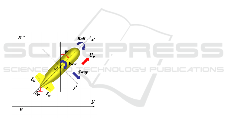
In treating the minimum-time guidance law, we use
two sets of coordinate systems: the inertial (earth-
fixed) coordinate system o-xy and the body fixed
coordinate system o'-x'y', as shown in Fig. 1.
Figure 1: Coordinate systems for optimal guidance problem
formulation.
As the marine vehicle used in our navigation problem,
we employ an autonomous underwater vehicle
(AUV) "r2D4" described in Kim and Ura (2009). In
Figure 1, actuator inputs as well as kinematic
variables used in the lateral dynamic model of our
AUV are represented. While
δ
pr
denotes the main
thruster axis deflection,
δ
el
and
δ
er
are the deflections
of elevators on left and right sides, respectively.
Vehicle heading
ψ
is defined as the angular
displacement of the x'-axis relative to the x-axis. In
this work, we approximate that the direction of the
vehicle's advance velocity coincides with the x'-axis.
Since the distribution of a sea current is considered to
be deterministic in our research, current velocity is
described as a function of the position and time.
Therefore, on the assumption that the advance
velocity of a vehicle and the current velocity are
superimposable, the resultant vehicle velocity in a sea
current is expressed as
y,t)(x,vsinUyv
y,t)(x,ucosUxu
c0
c0
+==
+==
ψ
ψ
(1)
where u and v are the components of the vehicle
velocity relative to the inertial frame, U
0
is the
advance speed of the vehicle in still water, and u
c
and
v
c
are the components of current velocity at a given
position and time. It is noted that we assume U
0
is
constant throughout a mission, which corresponds to
the operating condition of letting the rpm of vehicle's
main thruster fixed.
Equation (2) shows the minimum-time guidance law
of a marine vehicle moving in a sea current (Bryson
and Ho, 1975). Detailed procedure deriving (2) are
well explained in Kim and Ura (2009). It is noted here
that if only deterministic, there is no restriction on the
type of the sea current in (2). That is, not only
stationary, but also time-varying sea current can be
applied to (2) in deriving the solution for optimal
navigation. This leads to one of the most powerful
aspect of our approach over many other path planning
algorithms based on combinatorial optimization.
y
u
cos-sin2
y
v
-
x
u
2
1
x
v
sin
c
2
ccc
2
∂
∂
∂
∂
∂
∂
+
∂
∂
=
ψψψψ
(2)
2.2 Numerical Solution Procedure
Equation (2) is a nonlinear ordinary differential
equation (ODE) for an unspecified vehicle heading
ψ
(t). If the functions u
c
(x,y,t) and v
c
(x,y,t) describing
current velocity distribution are differentiable as well
as deterministic, the solution of (2) seems to be
attainable with an initial value of
ψ
(t), in terms of an
appropriate numerical solution algorithm such as
Runge-Kutta. However in practice, with an arbitrary
initial heading a vehicle travelling by the guidance
law (2) does not reach the destination. More precisely,
the initial value of vehicle heading is not arbitrary, but
is to be assigned correctly, consisting of a part of the
solution. This is because (2) is derived from the
Euler-Lagrange equation, which is a typical example
of the two-point boundary value problem,
characterized by split boundary conditions in states
ICINCO 2018 - 15th International Conference on Informatics in Control, Automation and Robotics
434
and costates (Bryson and Ho, 1975). To obtain the
solution of a two-point boundary value problem, an
iterative solution procedure is usually required. The
most famous and commonly used numerical
procedures for such purpose are the shooting and the
relaxation methods (Press et. al, 1992). However,
direct applications of these methods to our minimum-
time navigation problem have significant difficulties.
In applying shooting method to a two-point boundary
problem in time domain, governing ODEs with
proper initial guesses should be integrated until
reaching the upper limit of the boundary. However,
as noticeable from its name, i.e., the minimum-time
navigation, our problem is a so-called free boundary
one, having unspecified upper limit in time domain.
In treating a free boundary problem by relaxation
method, on the other hand, the independent variable
should be transformed into a new one defined
between 0 and 1. Here, we can anticipate an intrinsic
serious difficulty in determining the stepsize in free
boundary problems. Properness of temporal grid
distribution ensuring convergence is initially
unknown and to know it is extremely difficult before
the end of a computation. Moreover, strong initial
guess dependency of the solution is another serious
concern in applying the relaxation method to our
problem, inappropriate selection of which possibly
leads to a local optimality or divergence (Press et. al,
1992).
As a new approach deriving the numerical solution of
the optimal guidance law (2), we presented a search
procedure which determines correct initial heading of
this two-point boundary value problem. Being named
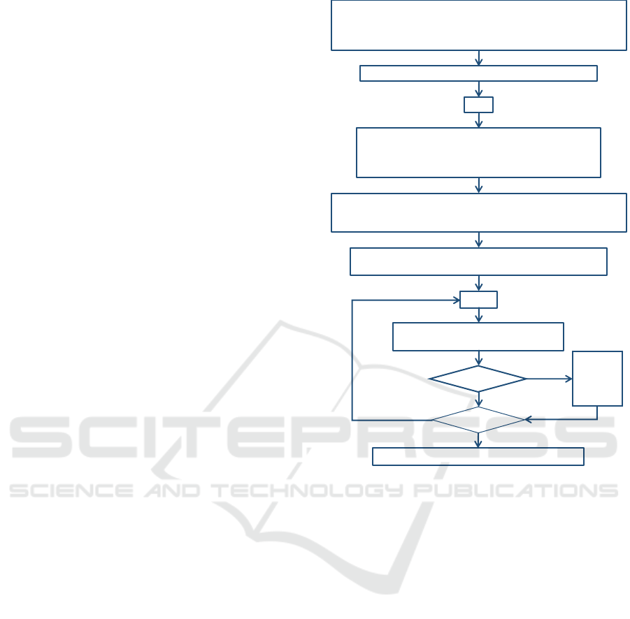
AREN (Arbitrary Reference Navigation), our
procedure works globally on the basis of the
minimum principle. Figure 2 shows the algorithmic
scheme of our solution procedure. In Fig. 2, an
asterisked variable denotes the one corresponding to
the optimal solution. Refer to Kim and Ura (2009) for
the details of AREN. By applying the correct (i.e.,
optimal) initial heading
ψ
0
*
derived by AREN to (2)
and solving it in time domain, we can obtain the time
sequence of the optimal heading reference which
achieves the minimum-time transit to the destination.
It is noted here that the minimum distance l
min
*
shown
in Fig.2 is to be interpreted as the residual error in the
converged solution, since it represents how closely a
vehicle has approached the destination. Therefore,
when l
min
*
is unacceptably large, the optimal initial
heading should be refined by further searches
repeated in the vicinity of
ψ
0
*
.
Figure 2: Algorithmic scheme of the numerical solution
procedure AREN for deriving the optimal initial heading.
3 SUBOPTIMAL NAVIGATION
3.1 Optimal Navigation Validation
As a validation test of our solution procedure
explained thus far, we conducted a simulation of
minimum-time vehicle routing in a stationary flow
field. Deterministic as it is, the flow field is an
artificial one induced by multiple vortical sources. A
vortical source is a mathematical singularity made of
a point source superimposed by a point vortex. Once
its location and strength are determined, flow field
induced by a vortical source is immediately
calculated (Kim and Ura, 2009). Locations and
strengths of the vortical sources used in this example
are summarized in Table 1.
In this example, the AUV r2D4 is routed by three
different navigation strategies. The first one is so
called proportional navigation (PN), which might be
the simplest strategy for guiding a vehicle to a target.
Apply any navigation (e.g., Proportional Navigation) to a vehicle
routing simulation in maneuvering the vehicle to reach the destination.
Keep the travelling time obtained as t
f_ref
, the reference final time.
Applied navigation is called the "Reference Navigation"
Prepare N equispaced heading guesses
ψ
i
within 0 ~ 2
π
.
i= 0
Make a vehicle routing simulation following the minimum-
time guidance law (2). The simulation continues until t =
t
f_ref
starting with the initial heading
ψ
0
= 0. This simulation
is referred to as 0-th trial.
i= i+1
Assign current minimum distance and reference final time to
their optimal values, i.e., , .
(0)
min
*
min
ll =
(0)
f_ref
*
f
tt =
Find the minimum distance between the destination and the
vehicle trajectory generated by the 0-th trial. is the travelling time
in the 0-th trial corresponding to the vehicle position of .
(0)
min
l
(0)
f_ref
t
(0)
min
l
Make i-th trial vehicle routing simulation
with the initial heading .
N / i2
(i)
0
π
ψ
=
?ll
*
min
(i)
min
≤
i= N-1 ?
(i)
min
*
min
ll =
(i)
0
*
0
ψ
ψ
=
Accept as approximate optimal initial heading.
*
0
ψ
Yes
Yes
No
No
)( i
f_ref
*
f
tt =
A Suboptimal Strategy for Autonomous Marine Vehicle Navigation in Variable Sea Currents
435
In PN, the heading of a vehicle is continuously
adjusted to let its line of sight (LOS) direct toward the
target. It should be noted here that, by default, PN is
used as the reference navigation deriving the
reference final time t
f_ref
(Fig. 2), in our research. The
second one used for the performance exemplification
of our optimal navigation is straight-line tracking. As
noticeable from its name, the straight-line tracking
lets a vehicle follow a straight-line trajectory
connecting the initial position and the destination. In
a straight-line tracking, vehicle heading is determined
so as to compensate for the trajectory normal
component of the flow velocity at current vehicle
position. Detailed descriptions as well as at-sea field
results of the straight-line tracking navigation are
found in Kim and Ura (2002). In this paper, it is
assumed that the main thruster rpm of the AUV r2D4
is controlled to keep its water-reference velocity to be
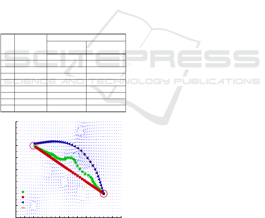
1.54 m/s throughout any mission. In Fig. 3, vehicle
trajectories in the vortical source flow field obtained
by three different navigation strategies are shown.
Table 1: Locations and strengths of vortical sources.
No. Location (m)
Vortical source strength
Source strength
(m
2
/s)
Vortex strength
(m
2
/s)
1 -50 , 250 -15 -10
2 -100 , 400 -40 -30
3 -100 , 500 -50 -50
4 -250 , 600 40 -35
5 -200 , 150 30 30
6 -300 , 350 -35 -35
7 -400 , 550 30 30
8 120 , 540 -40 60
9 -500 , 0 -50 15
Figure 3: Vehicle trajectories in a vortical source flow.
In each navigation shown above, the vehicle moves
towards the destination at the origin, starting from the
initial position (-400 m, 800 m). Though it gets to the
final state at the destination, the vehicle following PN
experiences severe drift due to the interaction with
current flow. In the straight-line tracking, the vehicle
has difficulty in moving toward the destination,
because in a large portion its travel, it is made to
advance against the flow. In the optimal navigation
however, the vehicle takes a detouring trajectory
riding on favorable flows. The optimal navigation
enables the vehicle to get flow-induced speed
increase in favorable flows. Travelling time reduction
by this speed increase prevails over the extra
travelling time caused by the detour, resulting in the
travelling times of 795.0 s, 762.5 s, and 550.5 s,
corresponding to the PN, straight-line tracking, and
optimal navigation, respectively.
3.2 Suboptimal Strategy
The optimal navigation implemented by our solution
procedure seems to work properly and effectively, as
shown in the previous example. Here, it should be
noted that one of the essential prerequisites for
accomplishing the proposed optimal navigation is
that the system being treated is deterministic. Induced
by mathematical singularities, vortical source flows
are perfectly deterministic without any uncertainty. In
real world, however, any measurement data does
contain uncertainty. Another significant issue is the
dynamic constraint. An optimal trajectory obtained
by solving the guidance law (2) is the one derived
without considering dynamic constraints of a specific
vehicle. This means that some optimal trajectories are
not able to be realized unless a vehicle exerts
unrealistic velocity or acceleration. As a remedy for
such issues, we propose the strategy of suboptimal
navigation. The suboptimal navigation is a fail-safe
strategy towards the field implementation of the
optimal navigation. The basic idea of the suboptimal
navigation presented in this paper is rather simple. Let
d
1
denote the deviation distance between the present
vehicle position and the preassigned one on the
optimal reference trajectory. When d
1
exceeds a
prescribed acceptable limit set for preserving an
ongoing optimal navigation, the high-level controller
for the vehicle navigation is activated and revises the
current optimal trajectory. By re-applying the AREN
to current vehicle position, velocity, attitude, as well
as environmental conditions, optimal trajectory as the
reference is newly revised. Figure 4 depicts the
schematic of the suboptimal navigation explained
thus far.
Lateral Posi tio n (m)
Longi t udinal Position (m)
-200 -100 0 100 200 300 400 500 600 700 800 900 1000
-600
-500
-400
-300
-200
-100
0
100
200
: Optimal Reference
: Propor t i opnal Navigation
: Straight-line Tracking
:Optimal(Tracked)
Initial Position
Destination
ICINCO 2018 - 15th International Conference on Informatics in Control, Automation and Robotics
436
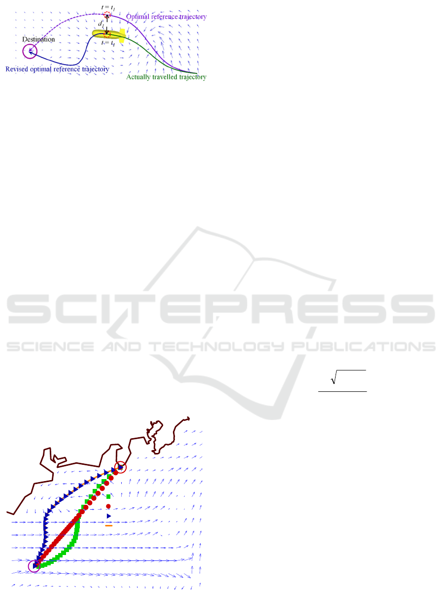
Figure 4: Schematic of the suboptimal navigation.
4 APPLICATIONS
4.1 Suboptimal Navigation in
Northwestern Pacific
In what follows, we apply the suboptimal navigation
to actual sea environments. The sea region selected
for the first example is located in the Northwestern
Pacific Ocean near Japan. The daily updated sea
current data of this region is available at https://www.
data.jma.go.jp/kaiyou/data/db/kaikyo/daily/current_
HQ.html?areano=2 presented by the Japan
Meteorological Agency. The most notable
environmental characteristic in this sea region is the
current field dominated by the Kuroshio. The
Kuroshio is a strong western boundary current
flowing northeastward along the coast of Japan.
At first, the optimal navigation has been applied to the
vehicle routing in the abovementioned sea region. In
this example, we do not consider any environmental
uncertainty in the sea current data. Figure 5 shows the
vehicle trajectories obtained by three different
navigation strategies: PN, straight-line tracking, and
optimal navigation.
Figure 5: Vehicle trajectories in a Northwestern Pacific
Ocean region.
As shown in the figure, like the preceding example in
which exact values of current velocity and its
gradients are available anywhere in the region, the
vehicle tracks the optimal reference trajectory with a
negligibly small deviation. This indicates that our
strategy of optimal navigation is also valid in the
actual sea current data.
In the following example, we apply the optimal
navigation to a vehicle routing in the same sea region
that was used in the preceding example. The only
thing different from the preceding example is we
consider uncertainty in our sea current data in order
to enhance the reality of our optimal navigation. An
environmental uncertainty model is introduced in
determining sea current velocities. The uncertainty
components in the sea currents are expressed as
additive white Gaussian noise (AWGN). Taking the
sea current velocities in the Northwestern Pacific
Ocean used beforehand as the mean values, on-site
current velocities including uncertainty are given by
u
cs
(x,y,t) = u
c
(x,y,t) + e
u
(
σ
)
v
cs
(x,y,t) = v
c
(x,y,t) + e
v
(
σ
)
(3)
where u
cs
and v
cs
are the components of the on-site
current velocity, u
c
and v
c
are the components of the
deterministic current velocity taken from the database,
and e
u
(
σ
) and e
v
(
σ
) are the AWGNs with standard
deviation
σ
. As the parameter for specifying the value
of
σ
in a given navigation region, we introduce the
regional mean current speed U
cm
defined as
N
vu
U
N
1i
2
ci
2
ci
cm
=
+
=
(4)
where i denotes the index covering all grid nodes on
which the database-based current velocities are
defined. In Fig. 6, vehicle trajectories obtained by
optimal navigation applied to different levels of
velocity uncertainties are shown. When the level of
velocity uncertainty is such that
σ
= 2U
cm
, the optimal
trajectory derived without considering uncertainty
still seems to work acceptably. As a result, though
slightly deviating from the destination, the final
position of the vehicle remains in the vicinity of the
destination. When the level of velocity uncertainty
increases up to
σ
= 4U
cm
, however, following the
optimal trajectory can no longer make the vehicle
approach the destination, as shown. As was
demonstrated in this example, the optimal navigation
proposed in this research bears the risk of failure
which increases in proportion to the degree of
environmental uncertainty.
Tokyo
Kii
Peninsula
Mainstream of Kuroshio
Initial Position
(Minamiizu)
Boso
Peninsula
Izu Peninsula
: Straight-line Tracking
Destination
: Optimal Reference
: Propor t i onal Navigation
: Optimal (Tracked)
Pacific Ocean
A Suboptimal Strategy for Autonomous Marine Vehicle Navigation in Variable Sea Currents
437
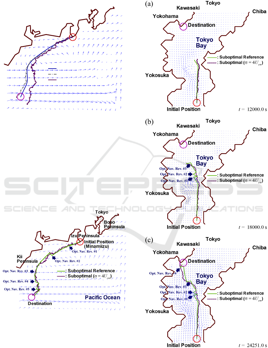
Figure 6: Vehicle trajectories in a Northwestern Pacific
Ocean region. In this example, on-site sea current velocities
are generated to include uncertainties expressed by
AWGNs.
Next, we apply the suboptimal navigation to a vehicle
routing in the same sea region. In the suboptimal
navigation, however, the vehicle does not merely
track the pregenerated optimal reference trajectory
throughout, but regenerates and follows new ones
whenever necessary, adapting to the current states of
environment as well as the vehicle position. Figure 7
shows the result of suboptimal navigation.
Figure 7: Vehicle trajectories by suboptimal navigation.
In Fig.7, it is noted that during the travel the optimal
navigation has been revised five times. Discontinuous
intervals appearing in the optimal reference trajectory
indicate the occurrences of the optimal navigation
revisions. These revisions enable the vehicle to arrive
at the destination.
Figure 8: Monitored vehicle trajectories by suboptimal
navigation in a tidal flow in Tokyo Bay observed at (a)
12000.0 s (b) 18000.0 s (c) 24251.0 s.
Tokyo
Kii
Peninsula
Pacific Ocean
Initial Position
(Minamiizu)
Boso
Peninsula
Izu Peninsula
:Optimal( )
Destination
: Optimal (without Uncertainty)
:Optimal( )
σ
σ U
cm
=4
=2U
cm
ICINCO 2018 - 15th International Conference on Informatics in Control, Automation and Robotics
438

4.2 Suboptimal Navigation in a
Time-Varying Sea Current
The last optimal navigation example presented in this
paper is an underwater vehicle routing in Tokyo Bay.
In this example, we consider the mission of
minimum-time homing to the port of Yokohama. Due
to its narrow entrance and shallow depth, sea currents
in Tokyo Bay are hardly affected by the outer ocean
currents such as Kuroshio. Instead, like many other
littoral zones, currents in Tokyo Bay are dominated
by the tidal flow. In this research, we use the time-
varying sea current distribution data in Tokyo Bay,
generated by a numerical tidal flow simulation model
by Kitazawa et al. (2001). Figures 8(a) ~ (c) are
sequential vehicle trajectories derived by applying the
suboptimal navigation. By the suboptimal navigation
consisting of total four self-revisions, the vehicle has
accomplished its homing mission.
5 CONCLUSIONS
In this paper, a systematic procedure for obtaining the
numerical solution of the optimal guidance law for a
marine vehicle moving in a region of sea current has
been presented. Reduced computational cost is one of
the outstanding features of our solution procedure.
Whilst linearly proportional to the area of a search
region in dynamic programming, the computational
time in our procedure exhibits square root
dependence on it. Moreover, unlike other path finding
algorithms such as dynamic programming or generic
algorithm, our procedure does not extend search
space when applied to a time-varying problem. This
means a great advantage that a time-varying problem
can be solved merely using the same computational
cost as is required for solving a time-invariant one.
As a fail-safe strategy for the field application of the
optimal navigation, suboptimal navigation has been
proposed. The fact that there actually are several
uncertainties which possibly disrupt ongoing optimal
navigation emphasizes the practical importance of the
suboptimal strategy proposed by us.
ACKNOWLEDGEMENTS
The author would like to thank Prof. D. Kitazawa of
IIS, the University of Tokyo for providing simulated
tidal flow data of Tokyo Bay.
REFERENCES
Nicholson, J. W., Healey, A. J., 2008. The present state of
autonomous underwater vehicle applications and
technologies. Marine Technology Society Journal,
42(1), 44-51.
Kim, K., Ura, T., 2010. Applied model-based analysis and
synthesis for the dynamics, guidance, and control of an
autonomous undersea vehicle. Mathematical Problems
in Engineering, 2010, Article ID 149385, 23 pages.
doi:10.1155/2010/149385.
Crespo L. G., Sun, J. Q., 2001. Optimal control of target
tracking with state constraints via cell mapping. J. of
Guidance, Control, and Dynamics, 24(5), 1029-1031.
Zhao, Y., Bryson, A. E., 1990. Optimal paths through
downbursts. J. of Guidance, Control, and Dynamics,
13(5), 813-818.
Alvarez, A., Caiti, A., Onken, R., 2004. Evolutionary path
planning for autonomous underwater vehicles in a
variable ocean. IEEE J. of Oceanic Engineering, 29(2),
418-429.
Papadakis, N. A., Perakis A. N., 1990. Deterministic
minimal time vessel routing. Operations Research,
38(3), 426-438.
Kamon, I., Rivlin, E., 1997. Sensory-based motion planning
with global proofs. IEEE Trans. on Robotics and
Automation, 13(6), 814-822.
Kim, K., Ura, T., 2009. Optimal guidance for AUV
navigation within undersea area of current disturbances.
Advanced Robotics, 23(5), 601-628.
Bryson, A. E., Ho, Y. C., 1975. Applied Optimal Control,
Taylor & Francis, Levittown.
Burken, J. J. et al., 2001. Two reconfigurable flight-control
design methods: Robust servomechanism and control
allocation. J. of Guidance, Control, and Dynamics,
24(3), 482-493.
McCormick, H., 2007. Reed's Nautical Almanac: North
American West Coast 2008, Thomas Reed Publications.
National Ocean Service, 2002. Tidal Current Tables 2003,
Pacific Coast of North America and Asia, International
Marine Publishing.
Robinson, A. R., 1999. Forecasting and simulating coastal
ocean processes and variabilities with the Harvard
Ocean Prediction System. In: Mooers, C.N.K. (eds.)
Coastal Ocean Prediction, 77-100.
Press, W. H., Flannery, B. P., Teukolsky, S. A., Vetterling,
W. T., 1992. Numerical Recipes in Fortran, Cambridge
University Press.
Kim, K., Ura, T., 2002. 3-dimensional trajectory tracking
control of an AUV "R-One Robot" considering current
interaction. In Proceedings of Int. Offshore and Polar
Engineering Conf., 277-283, Kita-Kyushu.
Kitazawa, D. et al., 2001. Predictions of coastal ecosystem
in Tokyo Bay by pelagic-benthic coupled model. In
Proceedings of 20th Int. Conf. on Offshore Mechanics
and Arctic Engineering, Rio de Janeiro, OSU-5035.
A Suboptimal Strategy for Autonomous Marine Vehicle Navigation in Variable Sea Currents
439
