Experimental Evaluation of Point Cloud Classiﬁcation using the PointNet

Neural Network

Marko Filipovi

c, Petra Ðurovi

c and Robert Cupec

Faculty of Electrical Engineering, Computer Science and Information Technology Osijek,

J. J. Strossmayer University, 31000 Osijek, Croatia

Keywords:

Point Cloud, Point Set, Point Cloud Classiﬁcation, PointNet, RGB-D, Depth Map.

Abstract:

Recently, new approaches for deep learning on unorganized point clouds have been proposed. Previous appro-

aches used multiview 2D convolutional neural networks, volumetric representations or spectral convolutional

networks on meshes (graphs). On the other hand, deep learning on point sets hasn’t yet reached the “matu-

rity” of deep learning on RGB images. To the best of our knowledge, most of the point cloud classiﬁcation

approaches in the literature were based either only on synthetic models, or on a limited set of views from

depth sensors. In this experimental work, we use a recent PointNet deep neural network architecture to reach

the same or better level of performance as specialized hand-designed descriptors on a difﬁcult dataset of non-

synthetic depth images of small household objects. We train the model on synthetically generated views of 3D

models of objects, and test it on real depth images.

1 INTRODUCTION

In this paper, classiﬁcation of objects in depth ima-

ges obtained by a 3D camera is considered. Object

classiﬁcation is the problem of categorization of an

object in the image in one of the previously deﬁned

classes according to similarity of its features to cer-

tain features characteristic to a particular class. Ob-

ject classiﬁcation is, for example, an important ca-

pability of an intelligent robot, which should handle

previously unseen objects. Classiﬁcation is also im-

portant for higher level tasks like object recognition.

Object recognition can also be referred to as object

detection, since normally it is desirable both to loca-

lize an object in a scene, whether its bounding box or

per-point mask, and to simultaneously determine its

class. Once we have a good classiﬁcation method, it

can be applied to object recognition using a sliding

box or a rough pre-segmentation method followed by

classiﬁcation.

RGB image classiﬁcation and related tasks on

RGB images have, arguably, already reached a ma-

ture state. Although classical methods like “hand-

designed” descriptors have proven useful, state-of-

the-art results were mostly obtained by deep neural

network-based methods. The benchmark example is

ImageNet dataset and related task of classiﬁcation of

RGB images into one of 1000 categories (classes)

(Russakovsky et al., 2015). Building on the success

of methods for RGB image modality processing, cor-

responding applications to point sets, i.e. unorgani-

zed point clouds

obtained from depth sensors, were

most often based either on a combination of RGB

and intensity-image classiﬁcation methods applied to

RGB and depth channels separately (for example (So-

cher et al., 2012); see (Cai, 2017) for more detailed

overview), or volumetric methods (for example (Wu

et al., 2015)), which encode a point set as a sparse

3D tensor. Viewing a depth image as an intensity

image and using corresponding 2D image patch pro-

cessing, as in convolutional neural networks (CNN-

s), however, doesn’t directly make use of geometric

properties of point sets. On the other hand, volume-

tric methods also have several problems: computatio-

nal complexity which quickly becomes high with in-

creasing resolution, quantization effect (point sets are

inherently non-uniform in density) and related pro-

blem of not-adapting to data density. Methods were

introduced that reduce the problem of computatio-

nal complexity of volumetric methods, but the main

problem still remained: none of these representations

is “native” to point sets, which results in the above

mentioned problems. Therefore, other types of re-

presentations for point sets were introduced. These

We will use the term point set in this paper to empha-

size the “unorganized” nature of point clouds.

Filipovi

c, M., Ðurovi

c, P. and Cupec, R.

Experimental Evaluation of Point Cloud Classiﬁcation using the PointNet Neural Network.

DOI: 10.5220/0006889200470054

In Proceedings of the 10th International Joint Conference on Computational Intelligence (IJCCI 2018), pages 47-54

ISBN: 978-989-758-327-8

include graph-based and point set-based representati-

ons. Graph-based representations are based on forma-

tion of a graph using local neighbourhood information

of points in the point set. Point set-based representa-

tions are the most general, since they don’t introduce

any prior information and instead use raw points. We

adopt such a representation in this work.

1.1 Contributions of this Paper

To the best of our knowledge, the existing point cloud

classiﬁcation approaches based on neural networks

were tested either only on 3D models (Qi et al.,

2017a; Qi et al., 2017b), on a limited set of views

from depth sensors (Socher et al., 2012) or using mul-

tiple views of an object (Qi et al., 2016; Su et al.,

2015). However, it is not clear how the classiﬁer trai-

ned on a limited number of views would generalize to

different views, which are not covered by the training

set. From our perspective, it is advantageous to have

3D models of objects to be able to synthetically gene-

rate every possible view, or, more precisely, all realis-

tic views of an object. On the other hand, we want to

test the classiﬁer on real RGB-D images. Therefore,

we train the network using many synthetically gene-

rated views of an object. Namely, we use a dataset of

3D models of objects, randomly rotate every model

multiple times, and capture partial views from a ﬁxed

virtual camera location. In this way, the model is ho-

ped to be general enough to be robust to viewpoint

variation. This also practically removes the need to

pre-align the models (i.e. depth maps) in both the

training and test sets. On the other hand, the model

is tested on real images from depth sensors. A similar

approach was used in a few papers before, for exam-

ple in (Song and Xiao, 2014), but not for our parti-

cular application: object classiﬁcation from a single

partial view, i.e. a depth map obtained from a depth

sensor.

We use the PointNet architecture (Qi et al.,

2017b), which has some important advantages com-

pared to commonly used volumetric methods, as dis-

cussed in the Introduction. Originally it was used only

for processing of full 3D models, but partial data in

the form of depth maps are more challenging.

We test this methodology on 3DNet (Wohlkinger

et al., 2012), a dataset of small household objects, and

obtain the same level of accuracy as the specialized

hand-designed descriptor (ESF) (Wohlkinger et al.,

2012; Wohlkinger and Vincze, 2011). However, one

of the advantages of neural network-based approaches

like the one we use here is speed

Actually, to be precise, here we refer to optimized GPU

implementations; as shown for example in (Ku et al., 2018),

1.2 Organization of the Paper

Related work is discussed in Section 2. PointNet (Qi

et al., 2017a) and PointNet++ (Qi et al., 2017b) neu-

ral network architectures for processing of point sets,

as well as data preparation procedure and training de-

tails, are reviewed in Section 3. The datasets used in

the experiments, the experimental setup and the obtai-

ned results are presented in detail in Section 4. Con-

cluding discussion can be found in Section 5.

2 RELATED WORK

Classiﬁcation methods based on RGB and intensity

image-based representations of RGB-D images in-

clude Convolutional-Recursive Neural Networks (So-

cher et al., 2012) and Multiview CNN-s (Qi et al.,

2016; Su et al., 2015). They share the common

ﬂaws of this type of methods, mentioned in the intro-

duction. Volumetric representations were studied for

example in (Maturana and Scherer, 2015; Wu et al.,

2015; Qi et al., 2016). Methods that reduce the com-

putational complexity of volumetric representations

include (Engelcke et al., 2017; Li et al., 2016). Graph-

based deep learning has also been intensively resear-

ched in recent years (Kipf and Welling, 2016; Verma

et al., 2017; Simonovsky and Komodakis, 2017; Def-

ferrard et al., 2016; Monti et al., 2017; Bronstein

et al., 2017; Klokov and Lempitsky, 2017). Point

set-based representations include (Qi et al., 2017a; Qi

et al., 2017b; Savchenkov, 2017; Monti et al., 2017;

Shen et al., 2017; Hua et al., 2017; Wang et al., 2018).

Regarding available datasets, here we review

some of the main representatives. ShapeNet (Chang

et al., 2015) is a large dataset of 3D models col-

lected from various places. It contains more than

3000 semantic categories and is an attempt to extend

the famous ImageNet (Deng et al., 2009) to 3D mo-

dels. Also, it contains rich annotations: language-

related (WordNet taxonomy), geometric (alignment,

part, symmetry, object size) and other. RGB-D Object

Dataset (Lai et al., 2011) contains RGB-D images of

300 objects from 51 categories. Since it contains non-

synthetic objects, it is well suited for testing classiﬁ-

cation algorithms on real data. It is (much) smaller

than ShapeNet, but still contains signiﬁcant number

of classes. It contains only a limited number of views

and, as discussed in Section 2, it s not clear how a

classiﬁer trained on this dataset would generalize to

different views. ModelNet (Wu et al., 2015) is anot-

her dataset of synthetic 3D models. It was used in

classical hand-crafted processing can potentially compete

with deep neural networks when implemented properly.

IJCCI 2018 - 10th International Joint Conference on Computational Intelligence

the literature both for 3D object and depth map, i.e.

partial view, classiﬁcation, as in (Maturana and Sche-

rer, 2015; Wu et al., 2015). The 3D models in Mo-

delNet are pre-aligned, which reduces the number of

degrees of freedom and makes the classiﬁcation task

easier. In addition to these, there are many other avai-

lable RGB-D datasets created for different purposes

(Firman, 2016), but for our application we found no

better dataset than 3DNet (Wohlkinger et al., 2012).

Namely, it contains 3D models of objects from diffe-

rent classes as the training set, and RGB-D images of

objects from the corresponding classes in the training

set.

A comprehensive literature review on 3D classi-

ﬁcation and recognition was done in (Carvalho and

Wangenheim, 2017). However, here we provided

more focused and, to the best of our knowledge, more

up-to-date references. Another recent performance

comparison of deep learning methods for RGB-D ob-

ject classiﬁcation can be found in (Cai, 2017). They

used a different methodology (more precisely, diffe-

rent point cloud representation and architectures of

neural network), and evaluated on different datasets.

3 METHODOLOGY

One of the ﬁrst methods for processing of raw point

sets was PointNet (Qi et al., 2017a). It is a deep

neural network that operates directly on point sets.

In the follow-up paper (Qi et al., 2017b), the impro-

vement of PointNet, named PointNet++, was introdu-

ced. PointNet processes a point set point-wise, and

doesn’t take into account neighbourhood information

around every point, as 2D convolution does. The main

idea of PointNet++ is to introduce local processing

into the PointNet architecture. However, extension

of 2D convolution to point sets is not straightforward

because of non-organized nature of point sets. Point-

Net++ doesn’t actually extend the 2D convolution to

point sets, but only applies PointNet architecture to

local point neighbourhood. However, it still proces-

ses local information hierarchically, and in that sense

is similar to 2D convolution. In many recent papers

(Monti et al., 2017; Shen et al., 2017; Hua et al., 2017;

Wang et al., 2018), various extensions of 2D convo-

lution to 3D point sets were proposed. Here we used

only the PointNet++ architecture for simplicity and

speed.

Historically, even networks with more than one hid-

den layer have been referred to as “deep”. Therefore, even

though we use less than 10 layers, as in the original Point-

Net architecture, we use the term deep network.

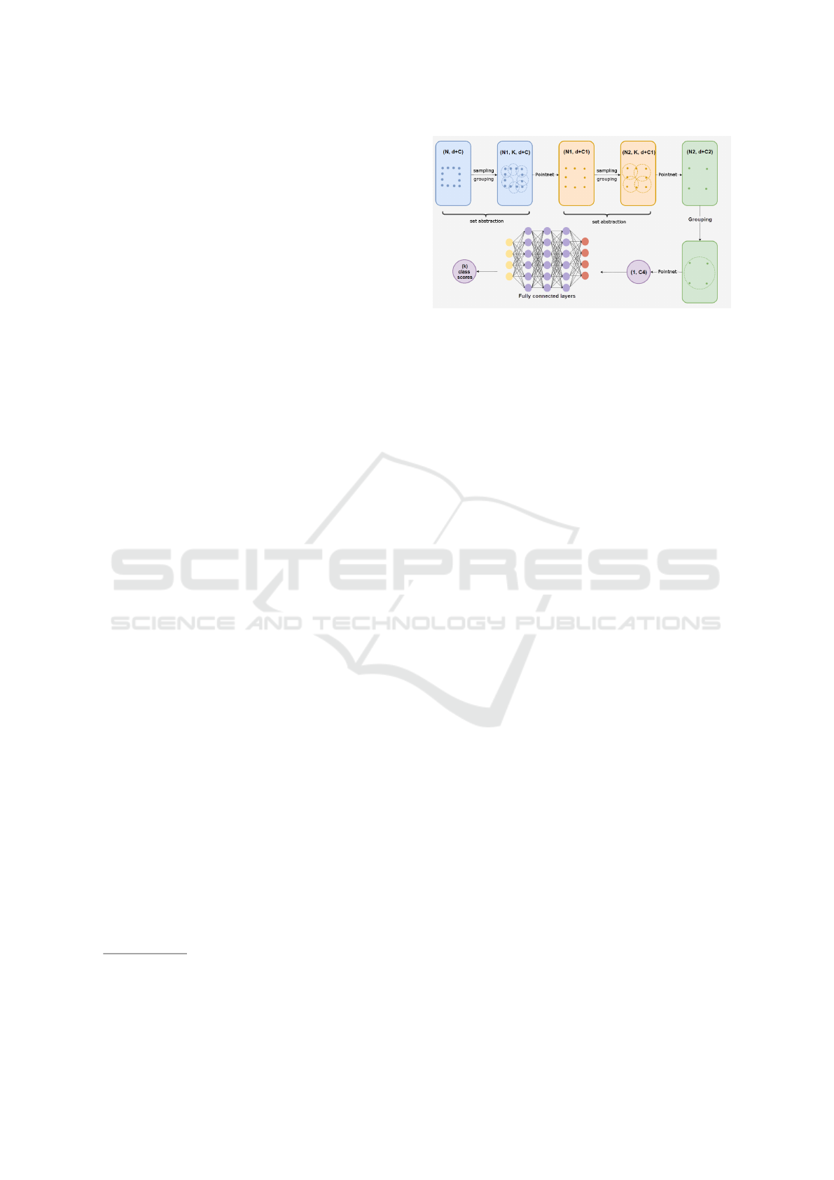
Figure 1: Architecture of PointNet++ network. N is the

number of points, d the input dimension, C the number of

input features (e.g. RGB or normals; we used C = 0), K the

number of nearest neighbours, N

the number of subsampled

points in layer i and C

is the number of channels of layer

i. Each pointnet layer operates ﬁrst pointwise, and ﬁnishes

with region-wise max pooling.

The overall architecture of PointNet++ is shown

in Figure 1. The ﬁrst part of the network serves as

a feature extractor. Its input is unorganized point

cloud, i.e. just a set of 3D points, optionally with

some features, like color or local surface normal for

every point. A very useful property of this network

is the invariance to the exact number and ordering

of input points. The output is a set of region (lo-

cal) features. This part consists of aggregation steps,

where points are grouped based on geometric distance

calculated from (x, y, z) coordinates and intermediate

PointNet-like layers which consist of convolutional,

Rectiﬁed Linear Unit (ReLU) nonlinearity and max-

pooling layers. The second part of the network is

basically a multi-layer perceptron (several fully con-

nected convolutional layers followed by ReLU), and

serves as a neural network classiﬁer. For more details

the reader is referred to the original paper (Qi et al.,

2017b).

The basic PointNet++ architecture, diagrammed

in Figure 1, can be improved by using multi-scale or

multi-resolution grouping. Here we brieﬂy describe

the multi-scale grouping (MSG). The reader is refer-

red to the original paper (Qi et al., 2017b) for more

details. Multi-resolution grouping was described as

more computationally efﬁcient in (Qi et al., 2017b),

but we use MSG here and sacriﬁce little speed for

accuracy. Neighbourhood grouping in PointNet++

can be performed in two basic ways: grouping based

on the number of nearest neighbours, and grouping

based on radius. We use grouping based on radius,

use multiple radii at each point, and concatenate the

resulting multiple features into one region-feature.

The notation we use to describe the ex-

act architecture used and its hyperparameters

is the following (it is the same as used in

Experimental Evaluation of Point Cloud Classiﬁcation using the PointNet Neural Network

the original paper (Qi et al., 2017b)). With

SA(K, [r

, . . . , r

], [[l

(1)

, . . . , l

(1)

], . . . , [l

(m)

, . . . , l

(m)

]])

we denote a multi-scale Set Abstraction (SA) layer

which groups input points into K regions (centered at

a subset of points selected using the Iterative Farthest

Point sampling), uses multiple scales with m radii r

with each scale followed by d per-point convolutional

pointnet layers, each having l

(i)

output channels

Per-point convolutional layers are all followed by

Rectiﬁed Linear Unit (ReLU) nonlinearity. Features

for m scales are concatenated into one l

(1)

+ . . . +l

(m)

region feature vector. Additional parameters should

be selected to account for the non-uniformity of

point sets: a number of points at every scale in every

neighbourhood. We add those as a third parameter to

the above deﬁnition of SA. SA ([l

, . . . , l

]) denotes

a global set abstraction layer that outputs a single

global feature. Basically, it is a set abstraction layer

that uses all points as one region. The output is then

an l

-element feature vector obtained by max-pooling

over all points. Fully connected layers are denoted by

FC(l, d p), where l is the width and d p denotes dro-

pout ratio. Fully-connected layers without dropout

are denoted by FC (l). The particular architecture

used in our research, as well as the values of all the

parameters, are presented in Section 4.

3.1 Preparation of Training Data

Here we describe the procedure for data preparation

and pre-processing used in the experiments.

For each instance in each class we generate a re-

asonably large number of synthetic views by rand-

omly rotating the model and capturing the view from

a ﬁxed virtual camera location. Our implementa-

tion of random rotation is based on Euler angles,

which doesn’t exactly cover the view sphere uni-

formly, but we consider it “uniform enough” to re-

present the views of an object from all angles. For

classes with smaller number of object instances, we

generate more views to make the training dataset ba-

lanced. A random subset of views, approximately ba-

lanced, is used as a validation set

during training for

early stopping. It should be noted that, in this way,

the stopping is done based on generalization to other

views of same instances and not to other instances.

We have tried using separate instances in each class

as a held-out validation set, but without improving the

Please refer to the original paper (Qi et al., 2017b) if

more clariﬁcations are needed.

That is, a held-out set which is not used in training and

serves as an indication of training progress in terms of ge-

neralization accuracy

results. Because we generate reasonably large num-

ber of views for each model, views in the validation

set are expected to be similar to some of the views in

the training set. However, it doesn’t seem to negati-

vely effect the generalizationn performance on the test

set, according to the obtained results. All point sets

are randomly subsampled to contain a ﬁxed number

of points, centralized, and normalized to unit sphere

prior to training. The same preprocessing is applied

to the validation and test sets. In (Wohlkinger et al.,

2012), a sub-sampling scheme based on the size of

mesh faces was used, which doesn’t assign all points

equal probability, but considering the relatively large

number of sampled points we use here, random sub-

sampling should sufﬁce.

3.2 Training Details

Robustness of deep neural networks, i.e. stability to

input perturbations is, unfortunately, not really their

known characteristic. This subject is an important to-

pic of current research, and many methods to achieve

robustness have already been proposed. Here we use

a common approach of input data augmentation: we

randomly perturb the input data during training, si-

mulating noise. More precisely, we split the training

process in two parts: in the ﬁrst part, we use no pertur-

bation, and train the network until the accuracy on the

validation set approximately reaches its maximum; in

the second part, we ﬁne-tune the resulting network

by perturbing the inputs both during training and va-

lidation, and again stop when validation accuracy on

the perturbed validation set approximately reaches its

maximum. Thereby, certain degree of stability to in-

put noise is achieved. Data augmentation as described

above also has another important purpose of reducing

the risk of overﬁtting.

We also note that previous works, e.g. (Song and

Xiao, 2014), have shown that it is advantageous to

train the model on synthetically generated views rat-

her than depth maps from depth sensors, due to sensor

noise and missing depth; namely, it improves the re-

sults on real depth maps compared to the model trai-

ned on noisy data only. Hence, we used the same stra-

tegy in our experiments.

4 EXPERIMENTS

We perform experiments on image clasiﬁcation on the

3DNet dataset (Wohlkinger et al., 2012). We used the

original code for PointNet++

. All experiments were

https://github.com/charlesq34/pointnet2

IJCCI 2018 - 10th International Joint Conference on Computational Intelligence

performed on a PC with 16GB RAM and with Nvidia

GeForce GTX 1060 GPU with 6GB memory.

3DNet dataset

contains 3 sets of CAD

models,

organized in 10 (Cat10), 60 (Cat60) and 200 (Cat200)

classes, respectively. Number of instance objects per

class varies. Since Cat10 model database contains

only colorless 3D models, only depth information is

used in our experiments. CAD models are generally

not aligned. For each instance in each class we gene-

rate 200 synthetic views, as described in Section 3.1.

In this way we obtain 15000 views per class for 10-

class 3DNet set. For larger, 200-class set, we generate

a smaller number (5000) of views per class. A random

subset of 10000 views is used as a validation set. All

point sets were randomly subsampled to contain 2048

points and preprocessed as described in Section 3.1.

Next, we describe the exact hyper-parameters of

the network. The following architecture was used for

the Cat10 dataset:

SA(256, [0.1, 0.2, 0.4], [32, 64, 128],

[[8, 16, 16], [16, 32, 32], [32, 64, 64]]) →

SA(64, [0.2, 0.4, 0.8], [16, 32, 64],

[[64, 64, 128], [128, 128, 256], [128, 128, 256]]) →

SA([256, 256, 256]) →

FC(256, 0.4) → FC(128, 0.4) → FC(10)

Also, batch normalization was used for all but the last

layer. We experimented with several combinations of

hyper-parameters, keeping the number of layers ﬁxed.

Also, we couldn’t reach the same accuracy with the

PointNet (Qi et al., 2017a) network, despite using the

same training procedure and hyperparameter-tuning.

Gaussian perturbations were added for data augmen-

tation, as described in Section 3.2, with standard devi-

ation 0.01. Optimization parameters were as follows:

initial learning rate was set to 0.001, with staircase

exponential decay every 200000 training samples and

decay rate of 0.7, and Adam was used as an optimiza-

tion algorithm with default values of exponential de-

cay rate for moments suggested in the original paper

(Kingma and Ba, 2014): β

= 0.9 and β

= 0.999.

Batch size was 32. The number of training epochs

was set to 200. The training took about 24 hours.

The test database in 3DNet consists of 1652 RGB-

D images of objects on the table, in various positi-

ons. Some of the images were corrupted, so we used

1612 of them for testing. The objects in the test ima-

ges are from the same set of classes as the training

https://repo.acin.tuwien.ac.at/tmp/permanent/3d-

net.org/

The acronym CAD refers to “Computer-Aided De-

sign”; here it means that the models are synthetically ge-

nerated.

set. Segmentation masks are not provided; therefore,

segmentation was performed as a preprocessing step.

Although object segmentation is not the topic of this

research, for the purpose of completeness, we provide

a brief explanation of the heuristic procedure used to

segment the objects of interest in the test images from

the background. Since the camera is mounted on a

ﬁxed position with respect to the scene, one image

is used to estimate the parameters of the supporting

plane and these parameters are then used to remove

the supporting plane from the other images. Further-

more, only the points within a cylindrical volume of

a speciﬁed radius around the camera were conside-

red. Then, connected sets of points, referred to in this

paper as clusters, were identiﬁed within this volume.

The object of interest is usually represented in the test

image by a single cluster, but in some cases it can be

split into two or more clusters. Hence, nearby clusters

are merged according to the proximity of their convex

hulls. Finally, the largest cluster is considered to be

the object of interest.

The results are shown in Table 1. The confusion

matrix can be seen in Table 2. Classes apple and

bowl are often confused, resulting in low accuracy on

apple class. However, other classes are discriminated

very well. The confusion matrix is similar to the one

in (Wohlkinger et al., 2012), where two classes are

confused and the rest are very well separated. Figure

2 shows examples of misclassiﬁed views on top of 3D

models from the predicted classes. In Figure 3 we also

show t-SNE (Maaten and Hinton, 2008) visualization

of features (before the fully connected layers) of point

clouds from the test set.

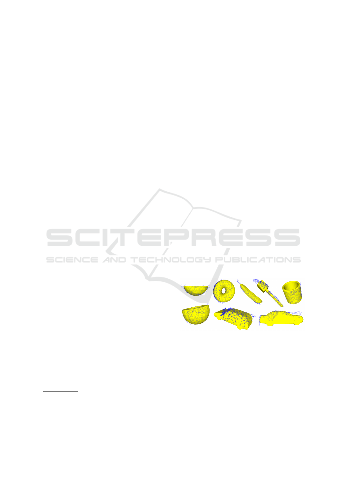
Figure 2: Examples of misclassiﬁed views, represented by

point clouds (blue points) on top of 3D models (yellow)

from the corresponding predicted classes. Left to right, top

to bottom: label apple, prediction bowl; label apple, pre-

diction donut; label bottle, prediction banana; label bottle,

prediction hammer; label toilet paper, prediction mug; label

mug, prediction bowl; label tetra-pak, prediction car; label

bottle, prediction car. Best viewed in color and zoomed in.

In overall, we get the same level of accuracy as

(Wohlkinger et al., 2012). The overall testing time for

1612 images in the test set, using our non-optimized

implementation, was 9 s. The testing speed is one of

the advantages of neural network-based classiﬁcation;

for example, in (Wohlkinger et al., 2012), the repor-

Experimental Evaluation of Point Cloud Classiﬁcation using the PointNet Neural Network

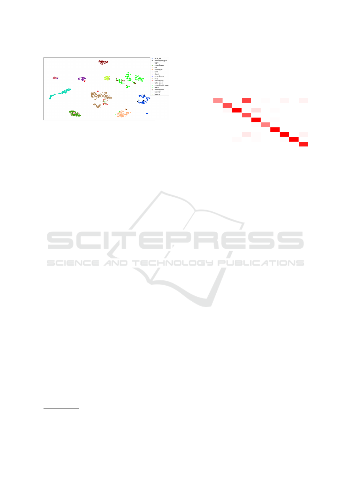
Figure 3: t-SNE visualization of features of point clouds

from the test set. missed_{class} denotes examples that

were misclassiﬁed by the network. Best viewed in color

and zoomed in.

ted processing time for one image is 45 ms, which

makes their method signiﬁcantly slower

. It should

be noted that most probably a better result could have

been obtained by generating (many) more views of

each object, and in a more formal manner, for exam-

ple by covering the 3D rotation parameter space uni-

formly and more densely. However, here we restricted

the training set to a reasonably large number of views

to make the training and hyperparameter tuning more

practical. Better results could possibly be obtained

by ﬁltering low-entropy views (i.e. non-informative /

non-realistic views) in the training and validation sets,

as in (Wohlkinger et al., 2012).

Table 1: Classiﬁcation accuracy on Cat10 subset of 3DNet

dataset. ESF refers to the descriptor that was used to obtain

the best results in (Wohlkinger et al., 2012), in combination

with 10-NN classiﬁer. OVERALL refers to average per-

class accuracy.

class ESF (Wohlkinger et al., 2012) our

apple 99% 35%

banana 89% 100%

bottle 94% 94%

bowl 88% 100%

car 98% 97%

donut 96% 98%

hammer 100% 100%

mug 100% 96%

tetra pak 91% 97%

toilet paper 61% 98%

OVERALL 92% 92%

The 3DNet dataset also contains a larger and more

difﬁcult Cat200 subset, with actually more than 200

classes. The overall accuracy reported in (Wohlkin-

ger et al., 2012) on that dataset is 71%. A signiﬁcant

hardware strength (most importantly, GPU memory)

and/or training time is needed to train the network for

Again, to be precise, hand-crafted processing can be

optimized for speed for real-time applications. Please see

footnote 2.

Table 2: Confusion matrix for the classiﬁcation on the

Cat10 dataset.

Predicted

apple

banana

bottle

bowl

car

donut

hammer

mug

tetra pak

toilet paper

Actual

apple

44 0 0 74 0 1 0 4 0 5

banana

0 69 0 0 0 0 0 0 0 0

bottle

0 3 307 0 13 0 1 0 0 0

bowl

0 0 0 68 0 0 0 0 0 0

car

0 0 0 0 153 0 1 0 0 0

donut

0 0 0 0 1 49 0 0 0 0

hammer

0 0 0 0 0 0 173 0 0 0

mug

0 0 0 9 1 0 0 357 0 5

tetra pak

0 0 2 0 1 0 0 1 168 0

toilet paper

0 0 0 0 0 0 0 0 0 90

such a large-scale dataset. Because of our hardware

limitations, we reduced the number of views per class

to 5000. This is probably the main reason why we

couldn’t reach the same level of accuracy. We show

the results on the Cat200 subset in Table 3.

Table 3: Classiﬁcation accuracy on Cat200 subset of 3DNet

dataset. ESF refers to the descriptor that was used to obtain

the best results in (Wohlkinger et al., 2012), in combination

with 10-NN classiﬁer. OVERALL refers to average per-

class accuracy. Please see the text for the explanation of

poor results on this subset and possibilities to improve them.

class ESF (Wohlkinger et al., 2012) our

apple 98% 0%

banana 70% 92%

bottle 79% 45%

bowl 76% 51%

car 44% 1%

donut 62% 78%

hammer 96% 50%

mug 99% 70%

tetra pak 72% 45%

toilet paper 17% 95%

OVERALL 71% 54%

The code for reproducing the results is available

upon request.

5 CONCLUSIONS

We have experimentally tested the promising point

set-based neural network acrhitecture PointNet on a

dataset of depth map images of small household ob-

jects. PointNet operates directly on unorganized point

clouds. The network is trained on synthetically gene-

rated views of 3D models of objects, and tested on

real depth images from depth sensor. We used only

geometric, i.e. depth information; no color informa-

tion was used. On the Cat10 subset of the 3DNet da-

taset, we obtained the same level of accuracy as the

IJCCI 2018 - 10th International Joint Conference on Computational Intelligence

original approach in (Wohlkinger et al., 2012), which

is, to the best of our knowledge, the best result on this

dataset. Neural network-based approaches, like the

one we used here, are, however, much faster. Also,

PointNet architecture was used mostly for processing

of full 3D data, and not partial scans, as we use it

here. On the Cat200 subset of the 3DNet dataset,

which is signiﬁcantly more computationally involved,

we couldn’t reach the same level of accuracy as re-

ported in (Wohlkinger et al., 2012); arguably, due to

GPU memory limitations. Generally, it would be inte-

resting to see a result analogous to those obtained on

the famous ImageNet classiﬁcation challenge, on a si-

milar dataset of 3D objects or depth scans from depth

sensors. We are aware of several related challenges

on the ShapeNet collection (Chang et al., 2015), but

not for classiﬁcation.

There are, of course, similar approaches to object

recognition and detection in scenes, also based on ge-

nerated views of 3D models of objects. However, they

are mostly based on volumetric or multi-view repre-

sentations, which can, arguably, be less practical in

certain applications. Also, here we were interested in

evaluating the performance on the specialized point

cloud classiﬁcation problem; namely, if a classiﬁca-

tion method performs well, especially the one based

on neural networks, it can be used as a basis for more

interesting problems of object detection (recognition)

in more complex scenes. For example, such approa-

ches were used for object detection in both RGB and

RGB-D images; however, that is still a very active

area of research.

ACKNOWLEDGEMENTS

This work has been fully supported by the Croa-

tian Science Foundation under the project number IP-

2014-09-3155.

REFERENCES

Bronstein, M. M., Bruna, J., LeCun, Y., Szlam, A., and Van-

dergheynst, P. (2017). Geometric deep learning: going

beyond euclidean data. IEEE Signal Processing Ma-

gazine, 34(4):18–42.

Cai, Z. (2017). Feature Learning for RGB-D Data. PhD

thesis, University of Shefﬁeld.

Carvalho, . L. E. and Wangenheim, . A. (2017). Literature

review for 3d object classiﬁcation/recognition.

Chang, A. X., Funkhouser, T., Guibas, L., Hanrahan, P., Hu-

ang, Q., Li, Z., Savarese, S., Savva, M., Song, S., Su,

H., et al. (2015). Shapenet: An information-rich 3d

model repository. arXiv preprint arXiv:1512.03012.

Defferrard, M., Bresson, X., and Vandergheynst, P. (2016).

Convolutional neural networks on graphs with fast lo-

calized spectral ﬁltering. In Advances in Neural Infor-

mation Processing Systems, pages 3844–3852.

Deng, J., Dong, W., Socher, R., Li, L.-J., Li, K., and Fei-Fei,

L. (2009). Imagenet: A large-scale hierarchical image

database. In Computer Vision and Pattern Recogni-

tion, 2009. CVPR 2009. IEEE Conference on, pages

248–255. IEEE.

Engelcke, M., Rao, D., Zeng Wang, D., Hay Tong, C.,

and Posner, I. (2017). Vote3Deep: Fast Object De-

tection in 3D Point Clouds Using Efﬁcient Convolu-

tional Neural Networks. In Proceedings of the IEEE

International Conference on Robotics and Automation

(ICRA).

Firman, M. (2016). Rgbd datasets: Past, present and future.

In Proceedings of the IEEE Conference on Computer

Vision and Pattern Recognition Workshops, pages 19–

31.

Hua, B.-S., Tran, M.-K., and Yeung, S.-K. (2017). Point-

wise convolutional neural network. arXiv preprint

arXiv:1712.05245.

Kingma, D. P. and Ba, J. (2014). Adam: A method for sto-

chastic optimization. arXiv preprint arXiv:1412.6980.

Kipf, T. N. and Welling, M. (2016). Semi-supervised clas-

siﬁcation with graph convolutional networks. arXiv

preprint arXiv:1609.02907.

Klokov, R. and Lempitsky, V. S. (2017). Escape from

cells: Deep kd-networks for the recognition of 3d

point cloud models. CoRR, abs/1704.01222.

Ku, J., Harakeh, A., and Waslander, S. L. (2018). In defense

of classical image processing: Fast depth completion

on the cpu. arXiv preprint arXiv:1802.00036.

Lai, K., Bo, L., Ren, X., and Fox, D. (2011). A large-scale

hierarchical multi-view rgb-d object dataset. In Robo-

tics and Automation (ICRA), 2011 IEEE International

Conference on, pages 1817–1824. IEEE.

Li, Y., Pirk, S., Su, H., Qi, C. R., and Guibas, L. J. (2016).

Fpnn: Field probing neural networks for 3d data. In

Advances in Neural Information Processing Systems,

pages 307–315.

Maaten, L. v. d. and Hinton, G. (2008). Visualizing data

using t-sne. Journal of machine learning research,

9(Nov):2579–2605.

Maturana, D. and Scherer, S. (2015). Voxnet: A 3d convo-

lutional neural network for real-time object recogni-

tion. In Intelligent Robots and Systems (IROS), 2015

IEEE/RSJ International Conference on, pages 922–

928. IEEE.

Monti, F., Boscaini, D., Masci, J., Rodola, E., Svoboda, J.,

and Bronstein, M. M. (2017). Geometric deep lear-

ning on graphs and manifolds using mixture model

cnns. In Proc. CVPR, volume 1, page 3.

Qi, C. R., Su, H., Mo, K., and Guibas, L. J. (2017a). Point-

net: Deep learning on point sets for 3d classiﬁcation

and segmentation. Proc. Computer Vision and Pattern

Recognition (CVPR), IEEE.

Qi, C. R., Su, H., Nießner, M., Dai, A., Yan, M., and Gui-

bas, L. J. (2016). Volumetric and multi-view cnns for

object classiﬁcation on 3d data. In Proceedings of the

Experimental Evaluation of Point Cloud Classiﬁcation using the PointNet Neural Network

IEEE Conference on Computer Vision and Pattern Re-

cognition, pages 5648–5656.

Qi, C. R., Yi, L., Su, H., and Guibas, L. J. (2017b). Point-

net++: Deep hierarchical feature learning on point sets

in a metric space. arXiv preprint arXiv:1706.02413.

Russakovsky, O., Deng, J., Su, H., Krause, J., Satheesh,

S., Ma, S., Huang, Z., Karpathy, A., Khosla, A.,

Bernstein, M., Berg, A. C., and Fei-Fei, L. (2015).

ImageNet Large Scale Visual Recognition Challenge.

International Journal of Computer Vision (IJCV),

115(3):211–252.

Savchenkov, A. (2017). Generalized convolutional neu-

ral networks for point cloud data. arXiv preprint

arXiv:1707.06719.

Shen, Y., Feng, C., Yang, Y., and Tian, D. (2017). Neig-

hbors do help: Deeply exploiting local structures of

point clouds. arXiv preprint arXiv:1712.06760.

Simonovsky, M. and Komodakis, N. (2017). Dynamic

edge-conditioned ﬁlters in convolutional neural net-

works on graphs. In Proc. CVPR.

Socher, R., Huval, B., Bhat, B., Manning, C. D., and Ng,

A. Y. (2012). Convolutional-Recursive Deep Learning

for 3D Object Classiﬁcation. In Advances in Neural

Information Processing Systems 25.

Song, S. and Xiao, J. (2014). Sliding shapes for 3d ob-

ject detection in depth images. In Fleet, D., Pajdla,

T., Schiele, B., and Tuytelaars, T., editors, Computer

Vision – ECCV 2014, pages 634–651, Cham. Springer

International Publishing.

Su, H., Maji, S., Kalogerakis, E., and Learned-Miller, E.

(2015). Multi-view convolutional neural networks for

3d shape recognition. In Proceedings of the IEEE

international conference on computer vision, pages

945–953.

Verma, N., Boyer, E., and Verbeek, J. (2017). Dynamic

ﬁlters in graph convolutional networks. arXiv preprint

arXiv:1706.05206.

Wang, Y., Sun, Y., Liu, Z., Sarma, S. E., Bronstein,

M. M., and Solomon, J. M. (2018). Dynamic graph

cnn for learning on point clouds. arXiv preprint

arXiv:1801.07829.

Wohlkinger, W., Aldoma Buchaca, A., Rusu, R., and Vin-

cze, M. (2012). 3DNet: Large-Scale Object Class Re-

cognition from CAD Models. In IEEE International

Conference on Robotics and Automation (ICRA).

Wohlkinger, W. and Vincze, M. (2011). Ensemble of shape

functions for 3d object classiﬁcation. In Robotics and

Biomimetics (ROBIO), 2011 IEEE International Con-

ference on, pages 2987–2992. IEEE.

Wu, Z., Song, S., Khosla, A., Yu, F., Zhang, L., Tang, X.,

and Xiao, J. (2015). 3d shapenets: A deep represen-

tation for volumetric shapes. In Proceedings of the

IEEE conference on computer vision and pattern re-

cognition, pages 1912–1920.

IJCCI 2018 - 10th International Joint Conference on Computational Intelligence