Deep Classifier Structures with Autoencoder for Higher-level Feature

Extraction

Maysa I. A. Almulla Khalaf

1,2

and John Q. Gan

School of Computer Science and Electronic Engineering, University of Essex,

Wivenhoe Park, CO4 3SQ, Colchester, Essex, U.K.

Department of Computer Science, Baghdad University, Baghdad, Iraq

Keywords: Stacked Autoencoder, Deep Learning, Feature Learning, Effective Weight Initialisation.

Abstract: This paper investigates deep classifier structures with stacked autoencoder (SAE) for higher-level feature

extraction, aiming to overcome difficulties in training deep neural networks with limited training data in high-

dimensional feature space, such as overfitting and vanishing/exploding gradients. A three-stage learning

algorithm is proposed in this paper for training deep multilayer perceptron (DMLP) as the classifier. At the

first stage, unsupervised learning is adopted using SAE to obtain the initial weights of the feature extraction

layers of the DMLP. At the second stage, error back-propagation is used to train the DMLP by fixing the

weights obtained at the first stage for its feature extraction layers. At the third stage, all the weights of the

DMLP obtained at the second stage are refined by error back-propagation. Cross-validation is adopted to

determine the network structures and the values of the learning parameters, and test datasets unseen in the

cross-validation are used to evaluate the performance of the DMLP trained using the three-stage learning

algorithm, in comparison with support vector machines (SVM) combined with SAE. Experimental results

have demonstrated the advantages and effectiveness of the proposed method.

1 INTRODUCTION

In recent years, deep learning for feature extraction

has attracted much attention in different areas such as

speech recognition, computer vision, fraud detection,

social media analysis, and medical informatics

(LeCun et al., 2015; Hinton and Salakhutdinov,

2006; Najafabadi et al., 2015; Chen and Lin, 2014;

Hinton et al., 2012; Krizhevsky et al., 2012; Ravì et

al., 2017). One of the main advantages of deep

learning due to the use of deep neural network

structures is that it can learn feature representation,

without separate feature extraction process that is a

very significant processing step in pattern recognition

(Bengio et al., 2013; Bengio, 2013).

Unsupervised learning is usually required for

feature learning such as feature learning using

restricted Boltzmann machine (RBM) (Salakhutdinov

and Hinton, 2009), sparse autoencoder (Lee, 2010;

Abdulhussain and Gan, 2015), stacked autoencoder

(SAE) (Gehring et al., 2013, Zhou et al., 2015),

denoising autoencoder (Vincent et al., 2008, Vincent

et al., 2010), and contractive autoencoder (Rifai et al.,

2011).

For classification tasks, supervised learning is

more desirable using support vector machines

(

Vapnik, 2013) or feedforward neural networks as

classifiers. How to effectively combine supervised

learning with unsupervised learning is a critical issue

to the success of deep learning for pattern

classification (Glorot and Bengio, 2010).

Other major issues in deep learning include the

overfitting problem and vanishing/exploding

gradients during error back-propagation due to

adopting deep neural network structures such as deep

multilayer perceptron (DMLP) (Glorot and Bengio,

2010; Geman et al., 1992).

Many techniques have been proposed to solve the

problems in training deep neural networks. Hinton et

al. (2006) introduced the idea of greedy layer-wise

pre-training. Bengio et al. (2007) proposed to train the

layers of a deep neural network in a sequence using

an auxiliary objective and then “fine-tune” the entire

network with standard optimization methods such as

stochastic gradient descent. Martens (2010) showed

that truncated-Newton method has the ability to train

deep neural networks from certain random

initialisation without pre-training; however, it is still

Khalaf, M. and Gan, J.

Deep Classiﬁer Structures with Autoencoder for Higher-level Feature Extraction.

DOI: 10.5220/0006883000310038

In Proceedings of the 10th International Joint Conference on Computational Intelligence (IJCCI 2018), pages 31-38

ISBN: 978-989-758-327-8

inadequate to resolve the training challenges. It is

known that most deep learning models are incapable

with random initialisation (Martens, 2010, Mohamed

et al., 2012, Glorot and Bengio, 2010b, Chapelle and

Erhan, 2011).

Effective weight initialisation or pre-training has

been widely explored for avoiding

vanishing/exploding gradients (Yam and Chow,

2000, Sutskever et al., 2013, Fernandez-Redondo and

Hernandez-Espinosa, 2001, DeSousa, 2016, Sodhi et

al., 2014). Using a huge amount of training data can

overcome overfitting to some extent (Geman et al.,

1992). However, in many applications there is no

large amount of training data available or there is

insufficient computer power to handle a huge amount

of training data, and thus regularisation techniques

such as sparse structure and dropout technique are

widely used for combatting overfitting (Zhang et al.,

2015, Shu and Fyshe, 2013, Srivastava et al., 2014).

This paper investigates deep classifier structures

with stacked autoencoder, aiming to overcome

difficulties in training deep neural networks with

limited training data in high-dimensional feature

space. Experiments were conducted on three datasets,

with the performance of the proposed method

evaluated by comparison with existing methods. This

paper is organized as follows: Section 2 describes the

basic principles of the stacked sparse autoencoder,

deep multilayer perceptron and the proposed

approach. Section 3 presents the experimental results

and discussion. Conclusion is drawn in Section 4.

2 STACKED SPARSE

AUTOENCODER, DEEP

MULTILAYER PERCEPTRON,

AND THE PROPOSED

APPROACH

2.1 Stacked Sparse Autoencoder

An autoencoder is an unsupervised neural network

trained by using stochastic gradient descent

algorithms, which learns a non-linear approximation

of an identity function (Abdulhussain and Gan, 2016,

Zhou et al., 2015, Zhang et al., 2015, Shu and Fyshe,

2013). Figure 1 illustrates a non-linear multilayer

autoencoder network, which can be implemented by

stacking two autoencoders, each with one hidden

layer.

Figure 1: Multilayer autoencoder.

A stacked autoencoder may have three or more

hidden layers, but for simplicity an autoencoder with

just a single hidden layer is described in detail as

follows. The connection weights and bias parameters

can be denoted as

] ; ; ;[

2121

bbWvectorisedWvectorisedw =

where

∈

is the encoding weight matrix,

∈

is the decoding weight matrix,

Rb ∈

the encoding bias vector, and

Rb ∈

is the

decoding bias vector.

For a training dataset, let the output matrix of the

autoencoder be

],...,,[

21 m

oooO =

, which is

supposed to be the reconstruction of the input matrix

],...,,[

21 m

xxxX =

, where

Ro ∈

and

Rx ∈

are the output vector and input vector of the auto-

encoder respectively, and m is the number of samples.

Correspondingly, let the hidden output matrix be

],..., ,[

21 m

hhhH =

, where

Rh ∈

is the hidden

output vector of the autoencoder to be used as feature

vector in feature learning tasks.

For the i

sample, the hidden output vector is

defined as

()

bxWgh

(1)

and the output is defined by

()

bhWgo

(2)

where

(

) is the sigmoid logistic function (1 +

 (−))



For training an autoencoder with sparse

representation, the learning objective function is

defined as follows:

()

Lp p

sparse

xo W

=++

−



(3)

where p is the sparsity parameter,

is the average

output of the j

hidden node, averaged over all the

IJCCI 2018 - 10th International Joint Conference on Computational Intelligence

samples, i.e.,



(4)

and  is the coefficient for L

regularisation (weight

decay), and  is the coefficient for sparsity control

that is defined by the Kullback-Leibler divergence:

()

pppKL

log1

log

−

−+=

(5)

The learning rule for updating the weight vector

(containing W

, W

, b

, and b

) is error back-

propagation based on gradient descent, i.e.,

WgradW ⋅−=Δ

. The error gradients with respect to

, W

, b

, and b

are derived as follows respectively

(Abdulhussain and Gan, 2016, Zhang et al., 2015):

/)(*.

)

)((

WmXHg

XOWgradW

′













−

+−+−=

(6)

mIHg

XOWgradb

/)(*.

)

)(((

′













−

+−+−=

(7)

/))(( WmHXOgradW

+−=

(8)

mIXOgradb /)(

−=

(9)

where 



(



)

=

(



)

.∗ [1 − 

(



)

] is the derivative

of the sigmoid logistic function,

I ]1,...,1,1[=

is a

one vector of size m and .* represents element-wise

multiplication.

2.2 Deep Multilayer Perceptron (DMLP)

A deep multilayer perceptron is a supervised

feedforward neural network with multiple hidden

layers (Glorot and Bengio, 2010). For simplicity,

Figure 2 illustrates a DMLP with 2 hidden layers only

(There are usually more than 2 hidden layers).

Figure 2: Deep multilayer perceptron (DMLP).

2.3 Proposed Approach

Training deep neural networks usually needs a huge

amount of training data, especially in high-

dimensional input space. Otherwise, overfitting

would be a serious problem due to the high

complexity of the neural network model. However, in

many applications the required huge amount of

training data may be unavailable or the computer

power available is insufficient to handle a huge

amount of training data. With deep neural network

training, there may also be local minimum and

vanishing/exploding gradient problems without

proper weight initialisation. Deep classifier structures

with stacked autoencoder are investigated in this

paper to overcome these problems, whose training

process consists of the following three stages:

1) At the first stage, unsupervised learning is

adopted to train a stacked autoencoder with

random initial weights to obtain the initial

weights of the feature extraction layers of the

DMLP. The autoencoder consists of N input

units, an encoder with two layers of K1 and K2

neurons in each hidden layer respectively, a

symmetric decoder, and N output units. Figure

3 illustrates its structure.

2) At the second stage, error back-propagation is

employed to pre-train the DMLP by fixing the

weights obtained at the first stage for its feature

extraction layers (W1 and W2). The weights of

higher hidden layers and output layer for feature

classification (W3, W4, and W5) are trained

with random initial weights. Figure 4 illustrates

how it works.

3) At the third stage, all the weights of the DMLP

obtained at the second stage are refined by error

back-propagation, without random weight

initialisation. Figure 5 illustrates how it works.

In our experiment, three methods are compared.

The first method, M1, is SVM (Vapnik, 2013) with

the output of the SAE encoder as input, the second

method, M2, is the pre-trained DMLP as shown in

Figure 4, and the third method, M3, is the DMLP after

refined-training as shown in Figure 5. Their

classification performances are evaluated on several

datasets.

Deep Classiﬁer Structures with Autoencoder for Higher-level Feature Extraction

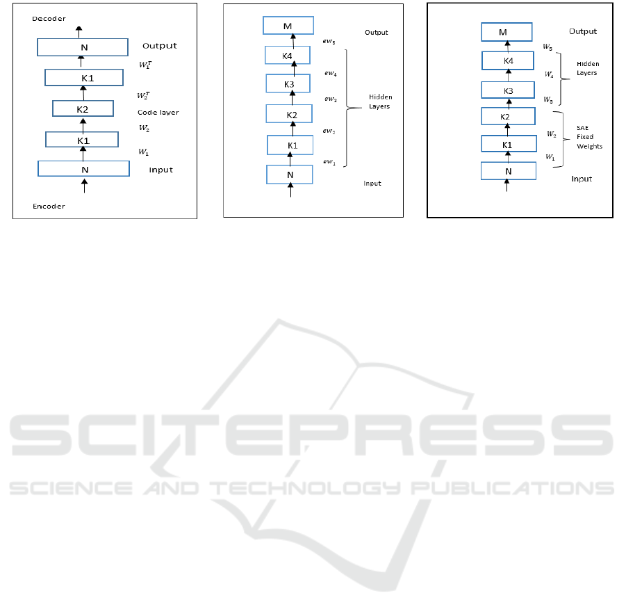
Figure 3: Training stacked

autoencoder (SAE).

Figure 4: Pre-training DMLP with

fixed W1 and W2 from SAE.

Figure 5: Refined-training of the

DMLP with initial weights from the

pre-trained DMLP.

3 EXPERIMENTAL RESULTS

AND DISCUSSION

3.1 Data Sets

Three document datasets were used in the experiments.

First, a phishing email dataset (http://snap.stanford.

edu/data/) has 6000 samples from two classes (3000

ham/non-spam and 3000 phishing), collected from

different resources such as Cornel University and

Enron Company. Second, the Musk dataset

(http://archive.ics.uci.edu/ml/ datasets.html) has 6598

samples from two classes (musk and non-musk). Third,

a phishing technical feature dataset (http://khonji.

org/phishing_studies) has 4230 samples from two

classes (2115 phishing and 2115 non-phishing).

The documents in these datasets were pre-

processed by tokenization, removing stop words such

as ‘the’, numbers and symbols, which helps to

produce a bag of words (BOW) as original features

(George and Joseph, 2014).

Term presence (TP) as weighting scheme was

then applied to the words in the BOW to obtain

numerical feature values (George and Joseph, 2014).

The total numbers of features for phishing emails,

Musk, and phishing technical feature datasets are 750,

166, and 47 respectively.

3.2 Experiment Procedure

Each dataset was partitioned into a training set and

a testing set. The training set was further partitioned

into estimation set and validation set for k-fold cross-

validation to determine the optimal or appropriate

network structure and hyper-parameter values (λ, β, p).

The proposed method was evaluated with

different number of hidden layers and different

number of hidden neurons during cross-validation,

and each testing set was only used once to evaluate

the performance of the proposed method with the

network structure trained using the hyper-parameter

values chosen by the k-fold cross-validation.

For a typical DMLP with 4 hidden layers, the

numbers of hidden neurons in the first stage are K1

and K2 respectively, and the numbers of hidden

neurons in the second or third stage are K1, K2, K3,

and K4 respectively. For training the SAE, 8 sets of

hyper-parameters (λ, β, p) were validated, as shown

in Table 1, which are around the suggested default

values.

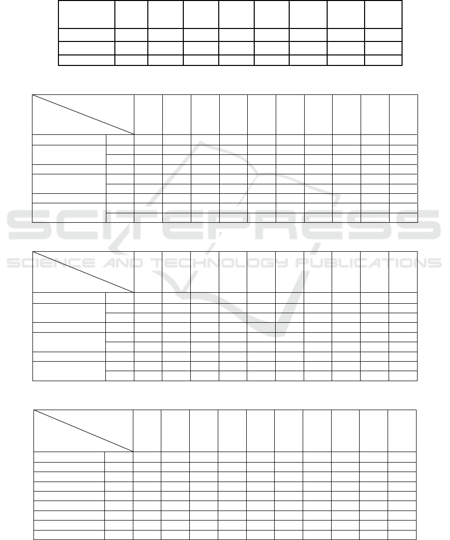
3.3 Results

1) Classification Accuracy: Tables 2-4 show the

cross-validation classification accuracies of the three

methods (M1, M2, and M3) with different hyper-

parameter values and different number of hidden

neurons, on the three datasets respectively. Tables 5-

7 show the corresponding training and testing

accuracies of the three methods with the appropriate

network structure trained using the hyper-parameter

values chosen by the cross-validation. Figure 6

compares the three methods in terms of average

training and testing accuracy. It can be seen from

Figure 6 that the proposed three-stage learning

algorithm for training deep classifier structures with

SAE, i.e., the M3 method, achieved the highest

accuracy, which have been proved to be statistically

significantly better than other methods evaluated in the

IJCCI 2018 - 10th International Joint Conference on Computational Intelligence

experiment. From Figure 6 it can be seen that the

proposed method (M3) has much smaller difference

between testing accuracy and training accuracy than

methods M1 and M2, which can be regarded as

evidence of less serious overfitting in the proposed

method. It can be concluded that DMLP with effective

weight initialisation can achieve significantly better

performance than the standard MLP, and it is evident

that the deep classifier structures with stacked

autoencoder can reduce overfitting.

Table 1: Hyper-parameters for training the SAE.

Hyper-

Parameters

HP1 HP2 HP3 HP4 HP5 HP6 HP7 HP8

L2W (λ)

0.001 0.001 0.001 0.001 0.001 0.01 0.1 0.5

Sp. Re. (

)

0 0 0 0 0 0 0 0

Sp. Pr. (

)

0.0005 0.005 0.05 0.5 1 1 1 1

Table 2: Cross validation accuracy on the phishing emails dataset.

Hyper-Parameters

Methods\

Network Structure

HP 1 HP 2 HP 3 HP 4 HP 5 HP 6 HP7 HP8 Ave

Acc.

Max

Acc.

SVM, 20 features M1 54.2 53.7 56.6 48.6 86.7 52.8 58.7 53.1 58.0 86.7

750-25-20-10-5-2

M2 88.7 88.9 86.8 89.8 87.9 88.9 87.1 88.4 88.3 89.8

M3 88.5 89.9 89.3 90.1 89.7 90.2 88.9 88.5 89.5 90.3

SVM, 25 features M1 51.6 76.3

89.2

62.2 47.4 77.7 54.3 49.1

63.4 89.2

750-50-25-15-10-2

M2 89.4 88.1 89.2 88.3 89.7

91.6

84.1 89.6

88.7 91.6

M3 91.7 90.6 89.3 91.1 90.5 90.5 90.9

92.4 90.7 92.4

SVM, 35 features M1 70.1 53.2 55.8 83.3 67.4 54.6 52.5 65.6 62.8 83.3

750-75-35-30-20-2

M2 88.1 88.2 88.8 88.9 88.5 88.4 88.9 89.2 88.6 89.2

M3 89.2 90.1 89.2 89.1 88.9 89.3 90.2 90.2 89.5 90.2

Table 3: Cross validation accuracy on the musk dataset.

Hyper-Parameters

Methods\

Network Structure

HP 1 HP 2 HP 3 HP 4 HP 5 HP 6 HP7 HP8 Ave

Acc.

Max

Acc.

SVM, 6 features M1 66.4 74.6 75.7 72.6 74.4 75.1 74.4 73.2 73.3 75.3

166-8-6-4-3-2

M2 77.0 78.8 78.8 90.8 83.2 86.1 96.1 77.1 83.5 96.0

M3 65.9 82.4 67.0 93.4 97.9 66.1 82.9 81.1 79.6 97.9

SVM, 7 features M1

75.4

74.7 58.7 74.0 74.1 74.9 74.2 61.7

70.7 75.4

166-10-7-5-3-2

M2 75.1 80.8 78.9 93.7

94.1

77.5 93.8 79.9

84.2 94.1

M3 83.0 86.0 79.5 90.1 83.2 76.7

98.9

79.7

84.9 98.9

SVM, 10 features M1 75.4 59.0 72.0 72.6 74.7 74.4 63.0 74.1 70.6 75.4

166-15-10-8-6-2

M2 77.7 81.3 79.8 95.2 93.8 77.8 92.1 80.8 84.8 95.2

M3 77.1 80.9 78.3 93.0 94.8 76.4 82.9 81.5 83.1 94.8

Table 4: Cross validation accuracy on the phishing technical feature dataset.

Hyper-Parameters

Methods\

Network Structure

HP 1 HP 2 HP 3 HP 4 HP 5 HP 6 HP 7 HP 8 Ave

Acc.

Max

Acc.

SVM, 6 features M1 54.2 54.2 57.7 54.2 59.6 60.4 60.5 55.7 56.3 60.4

47-8-6-4-3 M2 64.0 65.9 68.6 62.0 64.1 50.3 62.9 62.7 62.7 68.6

47-8-6-4-3 M3 97.0 96.3 89.0 90.8 97.7 96.7 96.8 96.8 95.1 97.7

SVM, 8 features M1 57.7 60.2 62.1 58.9

78.8

61.2 61.3 60.9

62.6 78.8

47-15-8-7-5-2 M2 66.0 66.9 64.5 63.1 64.0 59.9

90.5

62.8

67.2 90.5

47-15-8-7-5-2 M3 99.1 99.5

99.8

99.5 99.4 99.4 99.6 99.0

99.3 99.8

SVM, 15 features M1 57.2 58.6 58.6 51.1 58.8 58.6 58.5 57.7 57.3 57.7

47-30-15-10-6-2 M2 68.9 62.1 69.5 58.5 90.5 83.5 51.5 60.8 60.8 68.1

47-30-15-10-6-2 M3 99.4 99.3 99.3 99.1 51.1 84.3 99.3 99.1 91.1 99.4

Deep Classiﬁer Structures with Autoencoder for Higher-level Feature Extraction

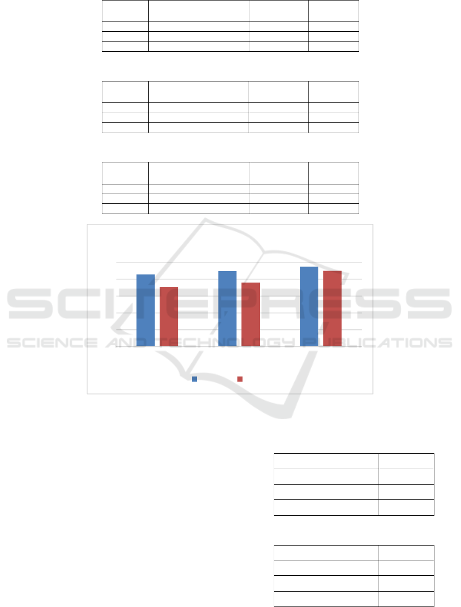
Table 5: Performance comparison on the phishing emails dataset.

Methods

Network Structure/

Hyper-Parameters

Training Acc. Testing

Acc.

M1 SVM, 25 features 85.2% 75.1%

M2 750-50-25-10-5-2/HP 6 90.7% 84.2%

M3 750-50-25-10-5-2/HP 8 92.6% 88.4%

Table 6: Performance comparison on the musk dataset.

Methods

Network Structure/

Hyper-Parameters

Training Acc. Testing

Acc.

M1 SVM, 7 features 87.3% 75.5%

M2 166-10-7-5-3-2/HP 5 95.2% 81.6%

M3 166-10-7-5-3-2/HP 7 98.1% 89.6%

Table 7: Performance comparison on the phishing technical feature dataset.

Methods

Network Structure/

Hyper-Parameters

Training Acc. Testing

Acc.

M1 SVM, 8 features 84.3% 61.8%

M2 47-15-8-7-5-2/ HP 7 83.1% 67.9%

M3 47-15-8-7-5-2/ HP 3 99.8% 91.8%

Figure 6: Comparison of the three methods in terms of average training and testing accuracy.

2) Statistical Significance Test: In order to assess

whether the performance differences among the

methods are statistically significant, we applied T-

test, a parametric statistical hypothesis test, and the

Wilcoxon’s rank-sum test, a non-parametric

method, to determine whether two sets of accuracy

data are significantly different from each other. The

statistical tests were conducted on three paired

methods (M3 vs M1, M3 vs M2, and M2 vs M1) in

terms of testing classification accuracy. Tables 8

and 9 show the p-values from these tests, which

demonstrate that, in terms of classification

performance, M3 significantly outperformed M1

and M2, and M2 significantly outperformed M1.

Table 8: Statistical test results (T-test).

Methods for comparison p-value

M3 vs. M1 6.9591e-05

M3 vs. M2 0.0013

M2 vs. M1 8.1148e-06

Table 9: Statistical test results (Rank-sum).

Methods for comparison p-value

M3 vs. M1 0.0345

M3 vs. M2 0.0576

M2 vs. M1 0.03241

100

M1 M2 M3

Training Testing

IJCCI 2018 - 10th International Joint Conference on Computational Intelligence

4 CONCLUSIONS

This paper investigates deep classifier structures

with stacked autoencoder for higher-level feature

extraction. The proposed approach can overcome

possible overfitting and vanishing/exploding

gradient problems in deep learning with limited

training data. It is evident from the experimental

results that the deep multilayer perceptron trained

using the proposed three-stage learning algorithm

significantly outperformed the pre-trained stacked

autoencoder with support vector machine classifier.

Also, it can be seen that the proposed method (M3)

has much smaller difference between testing

accuracy and training accuracy than methods M1

and M2, which can be regarded as evidence of less

serious overfitting in the proposed method.

Preliminary experimental results have demonstrated

the advantages of the proposed method. Further

tests on this algorithm would be applied to deep

neural networks with more layers and hopefully

would beef up the performance of these networks.

Also, tests with other applications would be

conducted in future investigations.

REFERENCES

Abdulhussain M.I. and Gan J.Q., 2016. Class specific pre-

trained sparse autoencoders for learning effective

features for document classification. Proceedings of

the 8th Computer Science and Electronic Engineering

Conference (CEEC), Colchester, UK, pp. 36-41.

Bengio Y., 2013. Deep learning of representations:

looking forward. Proceedings of International

Conference on Statistical Language and Speech

Processing, Spain. Lecture Notes in Computer

Science (LNCS), vol. 7978, pp. 1-37.

Bengio Y., Courville A., and Vincent P., 2013.

Representation learning: A review and new

perspectives. IEEE transactions on pattern analysis

and machine intelligence, 35, 1798-1828.

Bengio Y., Lamblin P., Popovici D., and Larochelle H.,

2007. Greedy layer-wise training of deep networks.

Proceedings of Advances in Neural Information

Processing Systems. MIT press, pp. 153-160.

Chapelle O. and Erhan D., 2011. Improved preconditioner

for hessian free optimization. Proceedings of the

NIPS Workshop on Deep Learning and Unsupervised

Feature Learning, pp. 1-8.

Chen X.W. and Lin X., 2014. Big data deep learning

challenges and perspectives. IEEE Access, vol. 2, pp.

514-525.

DeSousa C.A., 2016. An overview on weight

initialization methods for feedforward neural

networks. Neural Networks (IJCNN), International

Joint Conference , IEEE, 52-59.

Fernandez-Redondo M. and Hernandez-Espinosa C.,

2001. Weight initialization methods for multilayer

feedforward. Proceedings of European Symposium

on Artificial Neural Networks (ESANN), Bruges

Belgium, pp. 119-124.

Gehring J., Miao Y., Metze F., and Waibel A., 2013.

Extracting deep bottleneck features using stacked

auto-encoders. Proceedings of IEEE International

Conference on Acoustics, Speech and Signal

Processing (ICASSP), pp. 3377-3381.

George, K. and Joseph, S., 2014. Text classification by

augmenting bag of words (bow) representation with

co-occurrence feature. Journal of Computer

Engineering (IOSR-JCE), vol. 16, pp. 34-38.

Geman S., Bienenstock E., and Doursat R., 1992.Neural

networks and the bias/variance dilemma. Neural

Computation, vol. 4, pp. 1-58.

Glorot X. and Bengio Y., 2010. Understanding the

difficulty of training deep feedforward neural

networks. Proceedings of the 13th International

Conference on Artificial Intelligence and Statistics

(AISTATS), Sardinia, Italy, vol. 9, pp. 249-256.

Hinton G.E., et al., 2012. Deep neural networks for

acoustic modeling in speech recognition. IEEE Signal

Processing Magazine, vol. 29, pp. 82–97.

Hinton G.E., Osindero S., and Teh Y.W., 2006. A fast

learning algorithm for deep belief nets. Neural

Computation, vol. 18, pp. 1527-1554.

Hinton G.E. and Salakhutdinov R.R., 2006. Reducing the

dimensionality of data with neural networks. Science,

vol. 313, no. 5786, pp. 504-507.

Krizhevsky A., Sutskever I., and Hinton G.E., 2012.

ImageNet classification with deep convolutional

neural networks. Proceedings of Advances in Neural

Information Processing Systems, vol. 25, pp. 1090–

1098.

LeCun Y., Bengio Y., and Hinton G., 2015. Deep

learning. Nature, vol. 521, pp. 436-444

Lee H., Ng A.H., Koller D., and Shenoy K.V., 2010.

Unsupervised feature learning via sparse hierarchical

representations. Ph.D. Thesis, Dept. of Comp. Sci.,

Stanford University.

Martens J., 2010. Deep learning via Hessian-free

optimization. Proceedings of the 27th International

Conference on Machine Learning (ICML-10), pp.

735-742.

Martens J. and Sutskever I., 2012. Training deep and

recurrent networks with Hessian-free optimization. In

Neural Networks: Tricks of the Trade, Springer,

LNCS, pp. 479-535.

Mohamed A., Dahl G.E., and Hinton G.E., 2012.

Acoustic modeling using deep belief networks. IEEE

Transactions on Audio, Speech, and Language

Processing, vol. 20, pp. 14-22.

Najafabadi M.M., Villanustre F., Khoshgoftaar T.M.,

Seliya N., Wald R., and Muharemagic E., 2015. Deep

learning applications and challenges in big data

analytics. Journal of Big Data, vol. 2, no. 1, pp. 1-21.

Deep Classiﬁer Structures with Autoencoder for Higher-level Feature Extraction

Ravì D., et al., 2017. Deep learning for health informatics.

IEEE Journal of Biomedical and Health Informatics,

vol. 21, pp. 4-21.

Rifai S., Vincent P., Muller X., Glorot X., and Bengio Y.,

2011, Contractive auto-encoders: Explicit invariance

during feature extraction. Proceedings of the 28th

International Conference on Machine Learning, pp.

833-840.

Salakhutdinov R. and Hinton G.E., 2009. Deep

Boltzmann machines. Proceedings of the 12th

International Conference on Artificial Intelligence

and Statistics, Florida, USA, pp. 448-455.

Shu M. and Fyshe A., 2013, Sparse autoencoders for

word decoding from magnetoencephalography.

Proceedings of the 3

NIPS Workshop on Machine

Learning and Interpretation in NeuroImaging

(MLINI), Lake Tahoe, USA, pp. 20-27.

Sodhi S.S., Chandra P., and Tanwar S., 2014, A new

weight initialization method for sigmoidal

feedforward artificial neural networks. Proceedings

of International Joint Conference on Neural

Networks (IJCNN), Beijing, China, pp. 291-298.

Srivastava N., Hinton G., Krizhevsky A., Sutskever I.,

and Salakhatdinov R., 2014. Dropout: A simple way

to prevent neural networks from overfitting. Journal

of Machine Learning Research, vol. 16, pp. 1929-

1958.

Sutskever I., Martens J., Dahl G., and Hinton G.H., 2013.

On the importance of initialisation and momentum in

deep learning. Proceedings of the 30th International

Conference on Machine Learning, Atlanta, USA, pp.

1139-1147.

Vapnik, V. (2013). The nature of statistical learning

theory.Springer Science & Business Media.

Vincent P., Larochelle H., Bengio Y., and Manzagol P.A.,

2008. Extracting and composing robust features with

denoising autoencoders. Proceedings of the 25th

International Conference on Machine Learning, pp.

1096-1103.

Vincent P., Larochelle H., Lajoie I., Bengio Y., and

Manzagol P.A., 2010. Stacked denoising

autoencoders: Learning useful representations in a

deep network with a local denoising criterion. Journal

of Machine Learning Research, vol. 11, pp. 3371-

3408.

Yam J.Y.F. and Chow T.W., 2000. A weight initialization

method for improving training speed in feedforward

neural network. Neurocomputing, vol. 30, no. 4, pp.

219-232.

Zhang F., Du B., and Zhang L., 2015. Saliency-guided

unsupervised feature learning for scene classification,

IEEE Transactions on Geoscience and Remote

Sensing, vol. 53, no. 2, pp. 2175-2184.

Zhou X., Guo J., and Wang S., 2015. Motion recognition

by using a stacked autoencoder-based deep learning

algorithm with smart phones. Proceedings of

International Conference on Wireless Algorithms,

Systems, and Applications, pp. 778-787.

IJCCI 2018 - 10th International Joint Conference on Computational Intelligence