
Tracking Control of Electro-pneumatic Systems based on Petri Nets
Carlos Renato V´azquez
1
, Jos´e Antonio G´omez-Castellanos
2
and Antonio Ram´ırez-Trevi˜no
3
1
Tecnologico de Monterrey, Escuela de Ingenieria y Ciencias, Av. Ram´on Corona 2514, 45019, Zapopan, Mexico
2
UTZMG, Carr. Santa Cruz-San Isidro km. 45, 45640, Tlajomulco de Zu˜niga, Mexico
3
CINVESTAV Unidad Guadalajara, Av. del Bosque 1145, 45019, Zapopan, Mexico
Keywords:
Discrete Event Systems, Petri Nets, Automation.
Abstract:
This work introduces and solves a tracking control problem for electro-pneumatic systems (ENS) modeled
by interpreted Petri nets (IPN). The aim of this work is to maintain the si mplici ty of the specifications given
by practitioners in the field of ENS’s and formalize t he synthesis of a controller to ensure properties such as
controllability, liveness and boundedness. In order to achieve this goal, this work presents the IPN models for
ENS elements. The synchronous product of these modules yields in the plan model. Afterwards the synthesis
of the controller is presented as an algorithm that provides both an IPN model of the closed-loop system and
an IPN model of the controller, which can be translated to a Ladder Diagram for its implementation on a PLC
device. The method is applied to a small ENS to show its efficacy.
1 INTRODUCTION
Petri nets (PN) are a mathematical form alism useful
for modelling and analyzing discrete event systems
(DES), such as manufacturing system s, automation
systems, indu strial robotics, among others. The study
of PN’s has been particularly intensive for the synt-
hesis of controllers and supervisors. In the literature,
different supervision and contro l methods have been
reported for DES’s based on Petri nets. The most stu-
died control paradigms are :
• Supervisory-control (Ramadge and Wonham,
1987; Holloway et al., 1997; Iordache and Ant-
saklis, 2005). In this paradigm, the system be-
havior must be confined into the specification be-
havior (both given as lan guages) by me ans of a n
agent named supervisor that disabled controllable
events. The synthesis of the controller con sists in
the c omputatio n of the supreme controllable lan-
guage inside the specification, next, a DES that
generates such language is obtained and used as
the controller.
• Generalized mutual exclusions (Giua et al., 1992;
Basile et al., 2013). In this technique, places (na-
med monitors) an d arcs are ad ded to the PN, con-
straining the weighted sum of token s inside cer-
tain places. In this way, the behavior of the re-
sulting system avoids unsafe states or de a dlock
states; unsafe states are frequen tly either states in
which two activities occur simultaneously and in
deadlock states none transition is enabled.
• Liveness (Chen et al., 201 1; Li et al., 201 2). There
exist several works that address the problem of
controllin g the system in order to g uarantee its
liveness. Liveness is an important property ac-
cording to which, the firing o f any tran sition in
the future evolution is possible from any reacha-
ble state. In the literature, different analysis and
controller synthesis methods have been proposed
in order to guarantee liveness. Since the verifica-
tion of liveness is a NP problem in the number of
nodes, the studies frequently focus on net subclas-
ses, such as S3PR (Ezpeleta, 1995) , by using mat-
hematical programming (Li and Liu, 2007; Chao,
2009) or structural analysis (Li and Zhou, 2008;
S. Wang et al., 2012) to identify siphons that can
lose tokens, and then addin g mon itor places to
avoid that these siphons lose their tokens.
Despite the amount of works reported in the literature
regarding contro l techniques in PN’s, there is a lack of
theoretical developments and techniques for the synt-
hesis of controllers for different control objectives.
For instance, in the automation of industrial proces-
ses, the requirements are sequences of sensor s signals,
for which actuators must be executed in certain order;
in the control of flexible manufacturin g systems, the
requirements are pro cessed products, for which cer-
344
Vázquez, C., Gómez-Castellanos, J. and Ramírez-Treviño, A.
Tracking Control of Electro-pneumatic Systems based on Petri Nets.
DOI: 10.5220/0006861403440354
In Proceedings of the 15th International Conference on Informatics in Control, Automation and Robotics (ICINCO 2018) - Volume 1, pages 344-354
ISBN: 978-989-758-321-6
Copyright © 2018 by SCITEPRESS – Science and Technology Publications, Lda. All rights reserved

tain events must be executed, such as assemblies and
machine loads; in the supervision of rail tra nsport sys-
tems, the requirements are sequences of vehicle posi-
tions, for which the movement of the veh ic les is ena-
bled o r disabled in a safe mann er. In these applica-
tions, th e system is required to be con trolled in su c h
a way that its output be e qual to a refer ence signal.
The contr ol paradigms for DES’s mentioned above
do not address this problem . In fact, the design of
controllers for these a pplications is frequently based
on heuristic rules developed by practitioners, without
following any standard procedure that guarantee the
safe operation of the closed-loop system.
For these problems, the regulation control f rame-
work was introduced and studied in (Ram´ırez-Prado
et al., 2000; Santoyo et al., 2001; S´anchez-Blanco
et al., 2004; Campos-Rodr´ıguez et al., 20 04). In these,
the specification and the system to be controlled (the
Plant) are interpreted Petri nets (IPN), in which some
transitions are enabled or disable by mea ns of th e ap-
plication of certain input symbols, and some places
have symbols that are observable by external agents.
The objective is to design a controller that, for every
firing in the spec ification, executes a sequence of tr an-
sitions in the Plan t so the output symbols of the spe-
cification and the Plant become equal. In (Santoyo
et al. , 2001), the control method was illustrated in
an automation problem, including an algorithm for
translating the synthesized controller into a ladder di-
agram. Finally, in (Campos-Rodr´ıguez et al., 2004)
an extension of the control method was m a de in order
to consider partial observations.
In this work, the control of electro-pneumatic sys-
tems (ENS) is considered by using th e IPN paradigm.
From a practitioner point of view, the specification of
an ENS is given as a sequence of signals provided
by the actuators’ limit position sensors, such sequen-
ces are trigge red by signal from switches or proximity
sensors that are detecting the presence of parts or ma-
chine conditions. Nevertheless, in this kind of speci-
fications, not all ENS signals appe ar, or even worst,
some uncontrollable events may affect the plant, pro-
ducing sensor signals that not mentioned at the spe-
cification. Hence the con trol techniqu es repor te d in
the literature cannot handle these specifications. The
approa c h he rein presented, named Tracking Control,
handles these specificatio ns and synthesizes control-
lers capab le to drive the ENS behavior accord ing to
the specification, guaranteeing closed-loop properties
such as bounde dness and liveness.
To avoid overwhelming practitioners with the f or-
mal modeling of a plant, this work presents an IPN
model f or each ENS component. Since all the transiti-
ons are differently labeled, th en the synch ronous pro -
duct of these modules is merely the disjoint collection
of the pr e sented modules, simplifying the building of
the plant model. The specification is given as a simple
set of sequences o f IPN’s, where places h ave assigned
plant output symbols or are unlabeled. This specifica-
tion definition follows the idea of specifications given
by practitioners. The controller synthesis is presen te d
as an a lgorithm that can be easily followed, providing
both an IPN model of the closed-loop system and an
IPN model of the contr oller, which can be translated
to a Ladder Diagram for its implemen tation on a PLC
device.
This paper is organized as follows: in Section II
an overview of IPN’s is presented. In Section III,
IPN m odels for typical electron-pneumatic compo -
nents, and specifications, are introdu c ed. In Section
IV , the control synthesis algorithm is introduced , and
some properties of the clo sed-loop system are presen-
ted. In Section V , the introduce d co ncepts are illus-
trated through a case study. Conclusions and future
work are presented in Section V I.
2 BASIC CONCEPTS
In this section, the PN and IPN definitions and some
basic concepts are recalled (for more details see ( Da-
vid and Alla, 2010)).
2.1 Petri Nets
Definition 1. A Petri net (PN) structure N is a
bipartite digraph represented by the 4-tuple N =
hP,T,Pre,Posti where P = {p
1
, p
2
,..., p
n
} is the fi-
nite set of places, T = {t
1
,t
2
,...,t
m
} is the finite set
of transitions, Pre and Post are |P | × |T | matrices re-
presenting the weighted (nonnegative integer nu m ber)
arcs going from places to transitions and from transi-
tions to places, respectively. The incidence matrix of
N is defined as C = Post − Pre.
Let x ∈ P ∪ T be a node of N . The input set of
x, denoted by
•
x, is defined as
•
x = {x
i
∈ P ∪ T | there
exists an arc from x
i
to x}. Similarly, the output set of
a node x, denoted by x
•
, is define d as x
•
= {x
i
∈ P∪T |
there exists an arc from x to x
i
}.
A PN is a state machine if each transition has
only one input and one output plac e , i.e., ∀t ∈ T
|
•
t| = |t
•
| = 1 and it is strongly connected.
Definition 2. A PN system is the pair
N ,M
0
,
where N is a PN structure. The marking function
M : P → Z
+
is a mapping from each place to the no n-
negative integers representing the number of tokens
residing inside each place. The marking of a PN is
Tracking Control of Electro-pneumatic Systems based on Petri Nets
345

expre ssed as a column vector M of length |P|. M
0
is
the initial marking distribution.
The marking distribution evolves according to the fi-
ring of transitions. A transition t
j
is enabled at mar-
king M
k
iff ∀p
i
∈
•
t
j
, M
k
(p
i
) ≥ Pre(p
i
,t
j
), this is de-
noted as M
k
t
j
→. A transition t
j
can fire if it is ena-
bled. The firing of an enabled transition t
j
reaches
a new marking M
k+1
that can be computed with the
so-called PN fundamental equation
M
k+1
= M
k
+ Cv
k
where v
k
(i) = 0 for i 6= j and v
k
( j) = 1. This is deno-
ted as M
k
t
j
→ M
k+1
.
Graphically, places are represented by circles,
transitions by rectangles, arcs by arrows, and tokens
are represented as dots or positive integer numbers in-
side p la ces.
Definition 3. A sequence of transitions
σ = t
i
t
j
,...,t
k
of a PN system
N ,M
0
such
that M
0
t
i
−→ M
1
t
j
−→,..., M
w
t
k
−→ is said to be fireable or
it is said that σ is a firing transition sequenc e.
The marking M
′
reached after the firing of σ at a
marking M can be c omputed by
M
′
= M + C
~
σ
where
~
σ is a vector, named Parikh vector, defined as
a column vector of size |T | such that
~
σ( j) = k if t
j
is fired k times in the sequence σ. This is denoted as
M
σ
−→ M
′
, M
′
is said to be reachable from M.
The reachability set of a PN is the set of all the
reachable markings f rom M
0
, and it is den oted as
R(N ,M
0
).
A PN system is said to be bounded if the re ex-
ists a finite number k such that, for all the rea c ha-
ble markings, each place has a t most k tokens, i.e.,
∀M ∈ R(N ,M
0
) ∀p ∈ P it holds M(p) ≤ k. A PN
system is said to be safe if it is bounded with k = 1.
A PN system is said to be live if for any transi-
tion t
j
∈ T and any reachable marking M ∈ R(N ,M
0
)
there exists a fireable sequence σ such that M
σ
−→ M
′
and t
j
is enabled at M
′
.
2.2 Interpreted Petri Nets
In this work, the Interpreted Petri net model will be
used, which is a n extension to PN’s allowing to re-
present input and output symbols (Ram´ırez-Trevino
et al., 2003).
Definition 4. An Interpreted Petri net (IPN) system
is a 6-tuple Q =
N ,M
0
,Σ
I
,Σ
O
,λ, ϕ
where:
•
N ,M
0
is a Pe tri net system;
• Σ
I
is the input alphabet of the Petri net system,
where each element of the set Σ
I
is an input sym-
bol;
• λ : T → Σ
I
∪ {ε} is the labeling function o f
transitions with the restriction that nondeter-
ministic inputs are not allowed, i.e., ∀t
j
,t
k
∈
T, j 6= k, if Pre(p
i
,t
j
) = Pre(p
i
,t
k
) 6= 0 and both
λ(t
j
),λ(t
k
) 6= ε, then λ(t
j
) 6= λ(t
k
). Here, ε repre-
sents a system’s internal event;
• Σ
O
is the output alphabet of the Petri net system,
where each element of th e set Σ
O
is an output sym-
bol;
• ϕ : P → Σ
O
∪ {ε} is an output function that as-
sociates places to output symbols. ε represents a
symbol tha t is not available to an external obser-
ver.
The function ϕ can be represented by a |Σ
O
| × |P|
matrix ϕ, in which ϕ(i, j) = 1 if the place p
j
is asso-
ciated to the i-th output symbol and ϕ(i, j) = 0 other-
wise.
Here it is assumed that each place generates at
most one output symbol. A place p ∈ P is said to be
measurable if ϕ(p) 6= ε, otherwise, it is nonmeasura-
ble. A transition t is said to be controllable if λ(t) 6= ε,
otherwise it is uncontrollable .
The evolution of an IPN is similar to that of the
PN system with the addition that a symbol a ∈ Σ
I
is
indicated if it is activated by a n external device (for
instance a controller or a user). The f ollowing aspects
are also considered for the transitions firing.
• If λ(t
j
) = a
i
6= ε is indicated and t
j
is enabled then
t
j
must fire . If t
j
is enabled by the marking, but
the symbol λ(t
j
) is not indicated, then t
j
cannot
fire. If λ(t
j
) = ε and t
j
is enabled, then t
j
can fire
at any moment.
• At any reachable marking M
k
, an external obser-
ver reads the symbols associated to the marked
places.
In this work, it will be assumed that the IPN’s
are event-detectable (Ram´ırez-Trevino et al. , 2003),
a property that is recalled as follows:
Definition 5. An IPN
N ,M
0
,Σ
I
,Σ
O
,λ, ϕ
is said to
be event-detectable if the firing of any t
i
∈ T can be
detected by a change on the output symbols and can
be disting uished from the firing of other transitions,
i.e., ∀t
i
∈ T
• ϕC(•,t
i
) 6= 0
• ∀t
j
∈ T \{t
i
}, λ(t
i
) 6= λ(t
j
) or ϕC(•, i) 6= ϕC(•, j).
IPN models for complex systems can be built
from IPN submodels of in depende nt com ponents
ICINCO 2018 - 15th International Conference on Informatics in Control, Automation and Robotics
346

(i.e., the submodels do not share places, tra nsitions
or symbols). This is performed by the synchronous
product defined as follows:
Definition 6. Let Q
1
=
N
1
,M
1
0
,Σ
1
I
,Σ
1
O
,λ
1
,ϕ
1
and
Q
2
=
N
2
,M
2
0
,Σ
2
I
,Σ
2
O
,λ
2
,ϕ
2
be two IPN mo-
dels, where N
1
=
P
1
,T
1
,Pre
1
,Post
1
and N
2
=
P
2
,T
2
,Pre
2
,Post
2
. Th e synchronous product re-
sults in an IPN Q
3
N
3
,M
3
0
,Σ
3
I
,Σ
3
O
,λ
3
,ϕ
3
, where
where N
3
=
P
3
,T
3
,Pre
3
,Post
3
, denoted as Q
3
=
Q
1
||Q
2
. The IPN Q
3
is computed as follows:
• The net structu re is computed as follows: P
3
=
P
1
∪ P
2
and T
3
= T
1
∪ T
2
, enume rating first the
nodes in N
1
. Next, Pre
3
= diag(Pre
1
,Pre
2
) and
Post
3
= diag(Post
1
,Post
2
), where diag(•,•) is a
matrix built with the argument matrices as diago-
nal blocks, and other entries are null.
• The initial marking is M
3
0
= [(M
1
0
)
T
,(M
2
0
)
T
]
T
.
• The input and o utput alphabets are Σ
3
I
= Σ
1
I
∪ Σ
2
I
and Σ
3
O
= Σ
1
O
∪ Σ
2
O
, respectively.
• The input function is defined as: ∀t ∈ T
3
set
λ
3
(t) = λ
i
(t), where t is a node of T
i
with i ∈
{1, 2}. Similarly, the output function is defined
as: ∀p ∈ P
3
set ϕ
3
(p) = ϕ
i
(p), where p is a node
of P
i
with i ∈ {1,2}.
This synchronous product is compatible with the
previous reported in the litera ture since the IPN mo-
dules used in next sections are label disjo int (i.e. two
different modules do not share input symbols).
3 IPN PLANT AND
SPECIFICATION MODELS
In the f ollowing subsection, a library of IPN models
for the most frequently used components in ENS’s is
proposed; it inc ludes pu sh buttons, selectors, proxi-
mity sensors, electro-pneumatic valves and actuators.
In the next subsection , the plant model is built using
a bottom-up approach. It is very simple and appealing
from a practitione r point of view. Later, in Subsection
3.3, the specification mode l is defined.
3.1 Electro-pneumatic Component
Models
Figure 1 sh ows IPN models for different kind of swit-
ches. In these, output symbols are defined in the pla-
ces that represent a state in which the switch conducts
current. Figure 1. (a) repr esents a normally open (NO)
switch, whereas Figure 1.(b) represents a normally
closed (NC) switch. These switches can be either
push-buttons or switches (in such case, t
0
represents
the event o f “push” and t
1
the event of “rele ase”), or
lock-buttons (in such case, t
0
represents the event of
“push for the first time” and t
1
the event of “push for
the second time”). Figure 1.(c ) represents a single-
pole two-throw switch, in one state the current is con-
ducted to throw A, in the other state the current is con-
ducted to throw B. Finally, Figure 1.(d) represents a
selector betwee n three throws, A, B or C.
Figure 1: IP N models for different kinds of switches.
Figure 2 shows the electro-pneumatic symbols for
different kind of p roximity sensor s (DIN standard, as
used in electro-pneumatic diagrams) and its IPN mo -
del. All of them a re proximity sensors commonly
used in ENS’s to d etect a limit position of an actuator,
the presence of a part or a mach ine condition. These
sensors are the pressure sensor (Figure 2.(a)), the ca-
pacitive sensor (Figure 2.(b)), the inductive sensor
(Figure 2.(c)), the magnetic sen sor (Figure 2.(d)), and
the optical sensor (Figure 2.(e)). Frequently, these
sensors provide two output signals (in Figure 2 only
one terminal is drawn), o ne NO and one NC to detect
the pre sence and absence of parts, resp e ctively. For
that reason, the IPN m odel includes two output sy m-
bols, B for NC and A for NO. Transition t
0
represents
the event “a part is detected” and t
1
represents the
event “a part is not detected”. Reed magnetic sensors
(not shown) are used to detect limit positions of pneu -
matic actuators, these behave as NO switches, thus,
the model of Figure 1.(a) should be used for these sen-
sors.
Frequently, pneumatic actuators and valves are
used in usual assemblies, the most comm on are shown
in Figure 3 and Figure 4. Figure 3 shows a vacuum
actuator a ssembly, co nsisting of a 3-ways 2-positions
valve, a Venturi nozzle to produce vacuum, a suction
cup and a vacuum sensor, which provides an activa-
tion signal when vacuum is detected (when a pa rt is
grasped) . The IPN model of the vacuum assembly
represents the valve (nod e s p
3
, p
4
, t
3
and t
4
) and the
actuator (nodes p
0
, p
1
, p
2
, t
0
, t
1
and t
2
). Place p
0
re-
presents the state in wh ic h vacuum is n ot ac tivated,
thus the senso r pr ovides a signal B; p la c e p
1
repre-
Tracking Control of Electro-pneumatic Systems based on Petri Nets
347
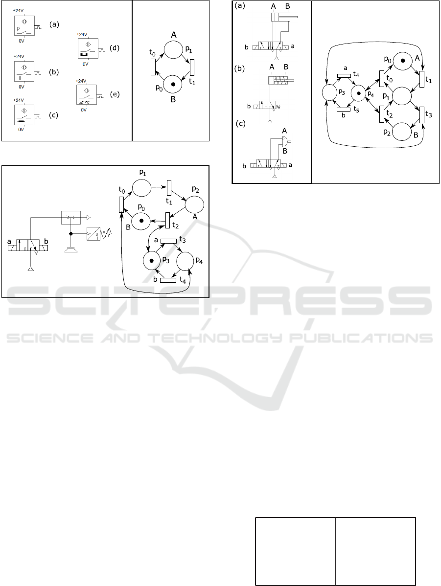
Figure 2: IP N models for different proximity sensors.
Figure 3: IP N model for vacuum assembly.
sents a transition state, and place p
2
represents the
state in which a part is grasped, thus the vacuum sen-
sor provides the output signal A. The activation of the
valve solenoids are the only controllable events, re-
presented by symbols a and b at transitions t
3
and t
4
,
respectively.
Figure 4 rep resents the most typical valve-actuator
assemblies: double acting actuator controlled b y a 5-
ways 2-positions valve (a), spring return actuator con-
trolled by a 3-ways 2-positions spr ing return valve
(b), and a rotary actuator controlled by a 5-ways 2 -
positions valve (c). Pneum a tic-grippers (not shown)
are usually driven by double acting actuators co ntrol-
led by 5-ways 2-positions valves, thus they are similar
to Figure 4.(a) . The same IPN model is valid fo r all
the assemblies. In this, the valve is represented by no-
des p
3
, p
4
, t
4
and t
5
, and the actuator is represented by
nodes p
0
, p
1
, p
2
, t
0
, t
1
, t
2
and t
3
. In the assemblies,
sensors are locate d to detect the limit positions, provi-
ding the ou tput signals represented by A and B, for the
leftmost and rightmost positions, respectively. On the
other hand, the activation of the valve solenoids are
the only controllable events, represented by symbols
a and b (to move to th e left a nd right, respectively)
at transitions t
4
and t
5
, respectively. For the case of
the spring return valve at Figure 4.(b), th e symbo l a is
Figure 4: IP N models for electro-pneumatic assemblies.
defined as the logical negation of b (i.e., the absence
of event b).
In addition to the introduced IPN models, the fol-
lowing control function must be stated. It ind ic a te s
the controllable transition that is ne eded to turn on a
particular sensor (i.e. to reach a marking where a me-
asurable place is marked). This is formalized in the
sequel:
Definition 7. The function t
→p
: P → T , which in-
dicates the controllable transition (if it exists) whose
firing leads to the marking of p, is defined as follows:
∀p ∈ P,
t
→p
(p) =
t if ϕ(p) 6= ε and there exists a d irected path
from a controllable transition t t o p, which
does not contain a n y other controllable
transition or measured place. If more than
one of such paths exists, then a ny of them
can be used,
t’ where t
′
∈
•
p, i f either ϕ(p) = ε or there
does not exist a path from a controllable
transition to p not containing oth er
measured places.
The models of figs. 1-2 do not contain controlla-
ble transitions, thus t
→p
is defined as in the second
statement of previous definition. For the models of
figs. 3 and 4, t
→p
is define d a s follows:
Model in Figure3 Model in Figure4
t
→p
(p
0
) = t
4
t
→p
(p
0
) = t
4
t
→p
(p
1
) = t
0
t
→p
(p
1
) = t
1
t
→p
(p
2
) = t
3
t
→p
(p
2
) = t
5
t
→p
(p
3
) = t
4
t
→p
(p
3
) = t
5
t
→p
(p
4
) = t
3
t
→p
(p
4
) = t
4
ICINCO 2018 - 15th International Conference on Informatics in Control, Automation and Robotics
348

3.2 Building the Plant Model
Following the Control Theory terminology, the sy-
stem to be controlled is named the Plant. A plant IPN
model for an ENS can be built by using the synchro-
nous product on the IPN models of the components.
Since the labels of the transitions are module disjoint,
then the plant is a disjoint collection of component
submodels (Figure 1-4). In other words, the plant mo-
del is a collection of disjoint ENS IPN modules.
Definition 8. The plant is a safe event-detec table
IPN Q
p
=
N
p
,M
p
0
,Σ
p
I
,Σ
p
O
,λ
p
,ϕ
p
, where N
p
=
hP
p
,T
p
,Pre
p
,Post
p
i, that models the DES to be con-
trolled. For an ENS with components {c
1
,.., c
n
}, its
plant IPN model can be obtained as follows:
• For each component c
i
, define its IPN model
Q
c
i
=
N
c
i
,M
c
i
0
,Σ
c
i
I
,Σ
c
i
O
,λ
c
i
,ϕ
c
i
, as shown in the
figs. 1-4, where N
c
i
= hP
c
i
,T
c
i
,Pre
c
i
,Post
c
i
i,
and define its function t
c
i
→p
. Different input and
output alphabets must be defined for different
compon ents, i.e., Σ
c
i
I
∩Σ
c
j
I
=
/
0 and Σ
c
i
O
∩Σ
c
j
O
=
/
0 if
j 6= i.
• The plant’s IPN m odel is computed as
Q
p
= Q
c
1
||...||Q
c
n
• The function t
p
→p
of the plant is computed as:
∀p ∈ P
p
set t
p
→p
(p) = t
c
i
→p
(p), where p is a node
of P
c
i
.
Moreover, Σ
act
O
⊆ Σ
p
O
is defined as the subset of output
symbols related to actuators (symbols from models of
Figure 3-4).
3.3 Specification Model
In ENS’s, specificatio ns are a collection of plant out-
put signals seque nces. In th em, neither th e occurr en-
ces of internal events nor the reachability of silent sta-
tes are specified.
Each specification sequence must include a strict
sequences of actuators’ output symbols that are requi-
red to occur in the plan t (sensor or switch plant output
symbols are allowed to occur in any or der). In these
sequences, a place p must be de fined for each instance
of a required p la nt outpu t symbo l o; this place must
have associated the symbol o. In a ddition, specifica-
tion sequences may have extra places with associated
symbols from sensors and switch e s, defining guard s
for the occurrence of sequences, which can be imple-
mented as either a place in the sequenc e or as self-
loop places.
In this work, the specification is represented as
an IPN describing output sequences and/or selections
between output sequences. This is formalized as fol-
lows:
Figure 5: IPN models of plant (a) and specification (b) of
example 1.
Definition 9. An specification is a safe and live state
machine IPN Q
s
=
N
s
,M
s
0
,Σ
s
I
,Σ
s
O
,λ
s
,ϕ
s
, with ad-
ditional marked self-loop places (a self-lo op is a
place p with Pre(p,t) = Post(p,t) = 1 for a particu-
lar transition t). All the transitions are c ontrollable.
The output alphabet of the specification is equal to the
output alp habet of the plant, i.e., Σ
s
O
= Σ
p
O
.
Example 1. For instance, consider an ENS con-
sisting of an assembly valve/double acting actuator
(the on e shown in Figure 4.a ), a proximity sensor
(shown in Figure 2) and a push button (shown in Fi-
gure 1.(a)). An specification for this system indica-
tes that when the proximity sensor detects a part the
actuator mu st complete two operation cycles (exten-
ding/returning).
The plant’s model is shown in Figure 5.(a), it is the
collection of the IPN models of each ENS component,
as expected. The specification is depicted in Figure
5.(b), notice that it is a sequence starting by symbol
A
s
and continuing with the two working cycle s of the
actuator, as th e required specification of the example
indicates.
Since the specification does not mention the plant out-
put symbols B
s
and A
b
, then they are not relevant fo r
the specific ation and can occur in an y order during
the plant’s operation. Moreover the sensor symbol
A
s
could occur in any order during the plant’s ope ra-
tion, however, the symbol A
s
is required to be p resent
for starting the sequenc e.
If the pressing of the push button is additionally re-
quired to start the seq uence, a self-loop place with
one token can be added to t
0
with the symbol A
b
, as-
sociated to the button’s closed position (i.e., a place p
connected with input an output arcs to t
0
, having one
token and the symbol A
b
).
Tracking Control of Electro-pneumatic Systems based on Petri Nets
349

4 CONTROL SYNTHESIS
ALGORITHM
The goal of the control of ENS’s is to drive the plant
in such a way that a required sequence of actuators’
movements is achieved, by activating the correspon-
ding valves, in response to the activation of sensors
and switches. At the IPN level th is means a proper sy-
nchronization of the plant and the specification. The
following algorithm provide s a formal solution for the
tracking control problem whenever the plant and the
specification are modelled according to Definitions 8
and 9. In the algorithm it is used the property ϕ(p) 6= ε
iff p is measured, similarly, λ(t) 6= ε iff t is co ntrolla-
ble.
Algorithm 4.1: Calculation of the closed-loop IPN and the
controller.
1: Input IPN models of the plant Q
p
and the speci-
fication Q
s
, and the function t
→p
.
2: Output IPN models of the c losed-loop system
Q
cl
and the co ntroller Q
c
.
% First, relabel the spec ification’s places as fol-
lows:
3: Let Σ
s
O
= {o
1
,..., o
m
} be the output alphabet of
Q
s
. Define a new output alphabet for Q
s
as Σ
s′
O
=
{o
′
1
,.., o
′
m
} and a bijective f unction Π : Σ
s
O
→ Σ
s′
O
such that Π(o
i
) = o
′
i
.
4: Define a new output function ϕ
s′
for the specifi-
cation as follows: ∀p ∈ P
s
,
ϕ
s′
(p) =
Π(ϕ
s
(p)) if ϕ
s
(p) 6= ε
ε otherwise
% Next, define mirror places in the specifica-
tion associated to places sharing the same output
symbol as follows:
5: Initialize P
s′
= P
s
, M
s′
0
= M
s
0
, Pre
s′
= Pre
s
and
Post
s′
= Post
s
.
6: for every p
i
∈ P
s
such that ϕ
s′
(p
i
) 6= ε do
7: if ∃p
j
∈ P
s
s.t. ϕ
s′
(p
i
) = ϕ
s′
(p
j
) then
8: Define the set of specification places with
the same output symbol as [p
i
] = {p
j
∈
P
s
|ϕ
s′
(p
i
) = ϕ
s′
(p
j
)}. Add a place p
′
i
to P
s′
.
Connect p
′
i
to other nodes in such a way that,
∀t
j
∈ T
s
, Pre
s′
(p
′
i
,t
j
) =
∑
p
s
∈[p
i
]
Pre
s′
(p
s
,t
j
)
and Post
s′
(p
′
i
,t
j
) =
∑
p
s
∈[p
i
]
Post
s′
(p
s
,t
j
).
9: Define th e initial marking of p
′
i
as M
s′
0
(p
′
i
) =
∑
p
s
∈[p
i
]
M
s
0
(p
s
). Therefor e, p
′
i
is marked iff
any place p ∈ [p
i
] is marked.
10: Define the output symbol ϕ
s′
(p
′
i
) = ϕ
s′
(p
i
).
Next, eliminate the output symbols from any
place in [p
i
].
11: end if
12: end for
13: Initialize the closed-loop system a s Q
cl
=
Q
p
||Q
s′
, where Q
s′
=
N
s′
,M
s′
0
,Σ
s
I
,Σ
s′
O
,λ
s
,ϕ
s′
and N
s′
= hP
s′
,T
s
,Pre
s′
,Post
s′
i.
% Next, add bidirectional arcs to Q
cl
, between
specification’s places and plant’s controllable
transitions, and between plant’s measured places
and specification’s transitions, as follows:
14: for every p
i
∈ P
s
such that ϕ
s′
(p
i
) 6= ε do
15: Let p
p
∈ P
p
be such that ϕ
p
(p
p
) = ϕ
s′
(p
i
). Let
t
j
= t
→p
(p
p
).
16: if λ
p
(t
j
) 6= ε then
17: Define a bidirectio nal arc between p
i
and t
j
,
i.e., set Pre
cl
(p
i
,t
j
) = Post
cl
(p
i
,t
j
) = 1.
18: end if
19: for every transition t
u
∈ p
•
i
do
20: Define a bidirectional arc between p
p
and t
u
,
i.e., set Pre
cl
(p
p
,t
u
) = Post
cl
(p
p
,t
u
) = 1.
21: end for
22: end for
23: The resulting IPN Q
cl
represents the clo sed-loop
system.
24: Initialize the IPN of the controller as Q
c
= Q
cl
.
25: Eliminate from Q
c
the plant’s nodes that are only
connected to o ther plant’s nodes, i.e., eliminate
places p ∈ P
p
s.t. Pre
c
(p,t) = Post
c
(p,t) = 0
∀t ∈ T
s
, and elim inate transitions t ∈ T
p
s.t.
Pre
c
(p,t) = Post
c
(p,t) = 0 ∀p ∈ P
s′
.
26: The resulting IPN Q
c
represents the controller.
Remark 1. Once th e controller Q
c
is computed by
the Alg orithm 4.1, it can be translated to a Ladder
Diagram as in (Santoyo et al., 2001) for its imple-
mentation in a PLC.
Example 2. Consider the plant of Figure 5. (a)
and the specification of Figure 5.(b). By apply ing
the Algorithm 4.1, the closed-loop model depicted
in Figure 6 is obtained. In this, the p lant and
specification are drawn in solid line, whereas the
nodes and arcs added by the Algorithm 4.1 are drawn
in dashed line. In particular, steps 3-4 relabel the
specification symbols, fro m A
s
, A
a
and B
a
to A
′
s
, A
′
a
and B
′
a
, respectively. Notice that there are two place s
with the symbols A
′
a
and B
′
a
, then steps 5-12 defin e the
new places drawn in dashed line with their input and
output arcs, one for the symbol A
′
a
and another for
the symbol B
′
a
. The symbols in brackets {•} represent
symbols that should be removed at step 9, but they are
kept in Figure 6 for this explanation. Notice that the
place with symbol A
′
a
(resp. B
′
a
) is marked iff any of
the places with symbol {A
′
a
} (resp. {B
′
a
}) is marked,
that is why they are called mirror places. Steps 15-18
add bidirectional arcs from the places with symbols
A
′
a
and B
′
a
to the plant’s controllable transitions with
ICINCO 2018 - 15th International Conference on Informatics in Control, Automation and Robotics
350
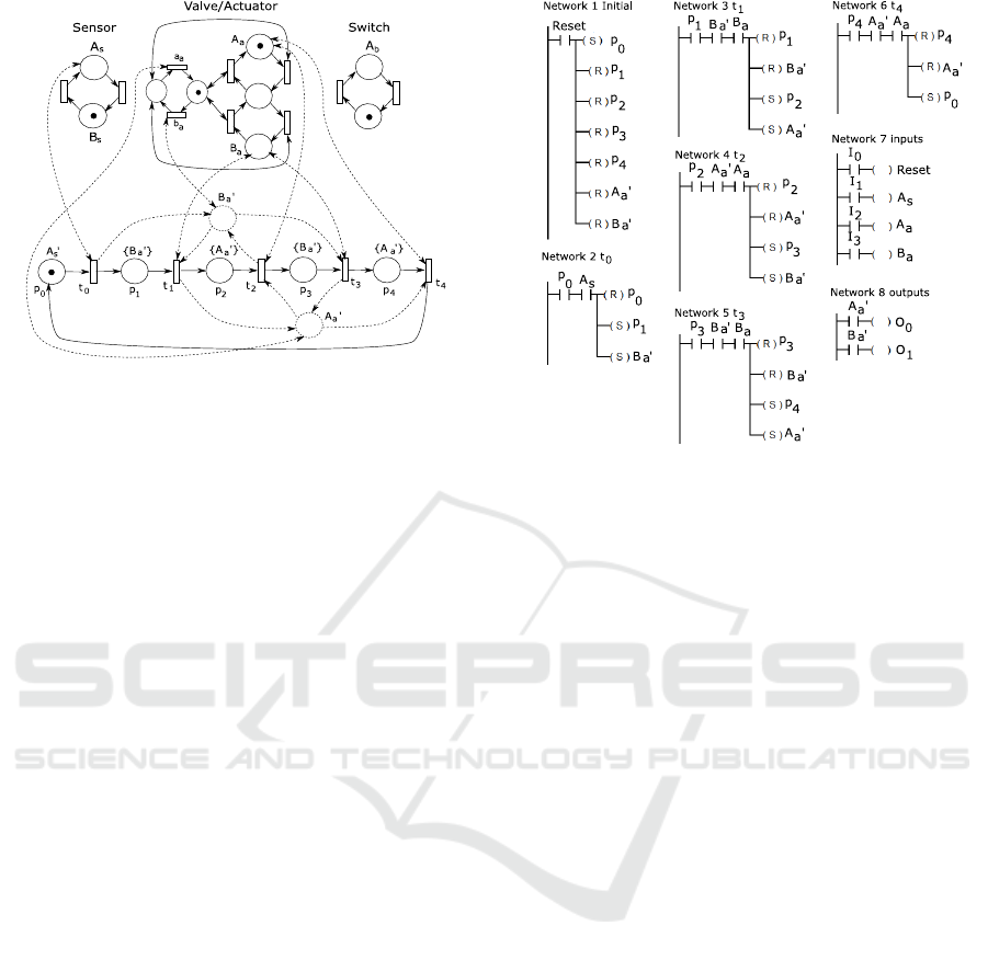
Figure 6: IP N closed-loop system of example 2.
symbols a
a
and b
a
, respectively. Steps 19-21 add
bidirectional arcs from the plant’s measured places
with symbols A
a
and B
a
to the output transitions of
the new p laces with symbols A
′
a
and B
′
a
, respectively.
A simulation of the closed-loop system can show that
the Pla nt evolves following the specification, i.e., it
performs a doub le cycle after the sensor detects a
part. Moreover, notice that the sensor and switch can
change their states during the actuator’s movement,
in accordance to the explanatio n of example 1.
The controller Q
c
, can be obtained from the
closed-loo p model by elimin ating the plant’s node s
that are only connecte d to other pla nt’s nodes. The re-
sulting IPN can be translated to the Ladder Diagram
shown in Figure 7, by following the procedure explai-
ned in (Santoyo et al., 2001), in which an in te rnal coil
is defined for each non-plant place (a coil is ON iff the
corresponding place has a token), a network is defi-
ned for the places’ initial condition which is executed
after pressing a reset push-button, a network is added
for each specific ation transition (Pre arcs are trans-
lated to NO switches and Reset coils, Post arcs are
translated to Set coils), and other networks are added
for de fining the PLC inputs and o utputs.
4.1 Properties of the Closed-Loop
System
The Algorithm 4.1 ensures that the closed-loop sy-
stem exhibits important good properties. This is for-
mally introduced in the following proposition.
Proposition 1. Consider a plant IPN model Q
p
and
an specification IPN model Q
s
, as in Definitions 8
and 9. Consider the IPN closed-loop model Q
cl
=
N
cl
,M
cl
0
,Σ
cl
I
,Σ
cl
O
,λ
cl
,ϕ
cl
as computed by the Algo-
rithm 4.1. The following statements hold:
Figure 7: Ladder Diagram for the controller Q
c
of example
2. The inputs I
0
, I
1
, I
2
and I
3
of the PLC are connected to
a NO reset push-button, the NO terminal of the proximity
sensor A
s
, the actuator’s limit sensor A
a
and the actuator’s
limit sensor B
a
, respectively. The outputs O
0
and O
1
of the
PLC are connected to the electro-valve’s coils correspon-
ding to a
a
and b
a
, respectively.
1. The Algorithm 4.1 is well defined , i.e., all the re-
quired information is available a nd the resulting
models Q
cl
and Q
c
are IPN’s.
2. Q
cl
is bounded.
3. The plant is connected to the sp ecification only
through measured sensors and controllable tran-
sitions. Formally, for any p ∈ P
p
and t ∈ T
cl
\ T
p
,
if ϕ
p
(p) = ε then Pre
cl
(p,t) = Post
cl
(p,t) = 0,
else Pre
cl
(p,t) = Post
cl
(p,t). For any t ∈ T
p
and p ∈ P
cl
\ P
p
, if λ
p
(t) = ε th e n Pre
cl
(p,t) =
Post
cl
(p,t) = 0 , else Pre
cl
(p,t) = Post
cl
(p,t).
4. The plant is only allowed to evolve in order to re-
ach the specification symbol. Formally, for any
reachable marking M
i
∈ R(N
cl
,M
cl
0
), if th ere ex-
ists t
i
∈ T
s
such that M
i
t
i
→ M
j
, where M
i
(p
j
) = 0
and M
j
(p
j
) > 0 for a place p
j
∈ P
s
with ϕ
s
(p
j
) ∈
Σ
act
O
, then there exists a fireable sequence σ
i
=
t
1
i
t
2
i
...t
r
i
, de scribing a marking trajectory M
j
t
1
i
→
M
1
j
t
2
i
→ M
2
j
...
t
r
i
→ M
r
j
, such that:
(a) t
1
i
,t
2
i
,...,t
r
i
∈ T
p
,
(b) M
r
j
(p
s
) > 0, where p
s
∈ P
p
is such that
ϕ
p
(p
s
) = ϕ
s
(p
j
),
(c) ϕ
act
M
j
≥ ϕ
act
M
1
j
≥ ... ≥ ϕ
act
M
r−1
j
, where ϕ
act
is the restriction of ϕ
cl
to the rows associated
to the symbols in Σ
act
O
,
(d) any other sequence σ
′
i
= t
′1
i
,...,t
′u
i
, describing a
Tracking Control of Electro-pneumatic Systems based on Petri Nets
351
trajectory M
j
t
′1
i
→ M
′1
j
...
t
′u
i
→ M
′u
j
, s.t. M
j
(p
s
) =
M
′1
j
(p
s
) = ... = M
′u
j
(p
s
) = 0, t
′1
i
,...,t
′u
i
∈ T
p
and λ
p
(t
1
i
)...λ
p
(t
r
i
) = λ
p
(t
′1
i
)...λ
p
(t
′u
i
), fulfills
ϕ
act
M
j
≥ ϕ
act
M
′1
j
≥ ... ≥ ϕ
act
M
′u
j
.
5. The specific ation cannot evolve until the plant re-
aches the specification symbol. Formally, for any
p
s
∈ P
s
such that ϕ
s
(p
s
) ∈ Σ
p
O
, let p
i
∈ P
p
be
s.t. ϕ
s
(p
s
) = ϕ
p
(p
i
), then Pre
cl
(p
i
,t) 6= 0 for any
t ∈ p
•
s
∩ T
s
.
6. The PN system
N
cl
,M
cl
0
is live.
The second statement of Proposition 1 is required
for the controller to be r ealized with a finite number of
resources. The third statement stands for the realiza-
tion of the controller: the only arcs allowed between
the plant and the rest of nodes are b idirectional ar cs
between measured plant’s places and transitions not
in the plant, and between controllable plant’s transiti-
ons and places not in the plant.
The fourth and the fifth statements of Proposi-
tion 1 stand for the fulfillment of the specification.
The third statement requires th at if a transition t
i
in
the specification is enabled, whose firing generates a
symbol ϕ
s
(p
j
) th a t belongs to the actuators’ alpha-
bet Σ
act
O
, then there is a fireab le sequence σ
i
involving
only plant’s transitions (con dition a)) that leads to a
marking in the plant that generates the same outpu t
symbol ϕ
s
(p
j
) (condition b)). During th e execution
of σ
i
, output symbols from actuators can disappear,
but the generation of new actua tors’ symbols is not al-
lowed (excepting ϕ
s
(p
j
), co ndition c)). Condition d)
is a controllability c ondition, i.e., if anothe r seq uence
σ
′
i
is fireable from the same marking M
j
by indica-
ting the same input symbols sequence λ
p
(t
1
i
)...λ
p
(t
r
i
),
then σ
′
i
does not produce new output actuator sym-
bols. The fifth statement requires that the specifica-
tion cannot evolve u ntil the plant has reached the same
output.
Remark 2. The tracking controller is neither a par-
ticular case of the supervisory-control theory nor of
the regulation control framework for a given sp ecifi-
cation, because in our setting the output langu age of
the controlled system is not included in the specifica-
tion’s output language. It might be possible to modify
the specification in order to make the output tracking
controller fit in the supervisory-control or regulation
frameworks, however, such adaptation would not be
trivial and would not fulfilled Definition 9.
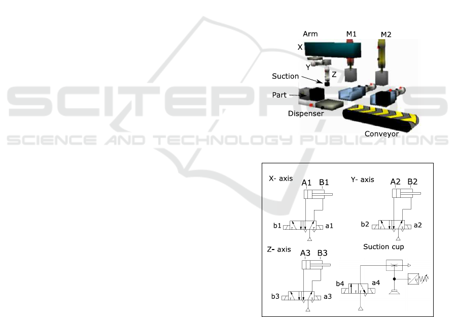
5 CASE STUDY
Consider the ENS depicted in Figure 8 composed of
one pneumatic arm, two stamping machines, on e part
dispenser, a conveyor and a start lock-button. The
ENS r equired functiona lity is the following. The
pneuma tic arm retrieves a part from the dispe nser and
loads it in the stamping machin e M
1
or M
2
, depending
on w hich is idle. Every tim e tha t a mach ine is loaded,
it stamps a nd forms the part. Whenever a machine
M
1
or M
2
finishes its work, the pneumatic arm unlo-
ads it placing the finished part on the conveyor. The
cycle is repe ated every time that the d isp enser h as a
part. The dispenser has a proximity sensor to indicate
that it ho lds a part (position As1) or it is empty ( posi-
tion Bs1); machines M
1
and M
2
have proximity sen-
sors to ind ic a te that the machine is idle without part
(positions B
s2
and Bs3 respectively) or they finished
a part that must be unloaded (po sitions As2 and As3
respectively).
Figure 8: ENS for case study.
Figure 9: Actuators for the electro-pneumatic arm.
In this section, the controller for the pne umatic
arm will be synthe sized. Its electro -pneumatic dia-
gram is shown in Figure 9. Every axis, X, Y, Z of
the pneumatic arm has an electro-pneumatic assem-
bly. The spe cification for the arm is composed of four
sequences, representing when the pneumatic arm: it
loads machine M
1
; it loads M
2
; it unloads M
1
; and it
ICINCO 2018 - 15th International Conference on Informatics in Control, Automation and Robotics
352
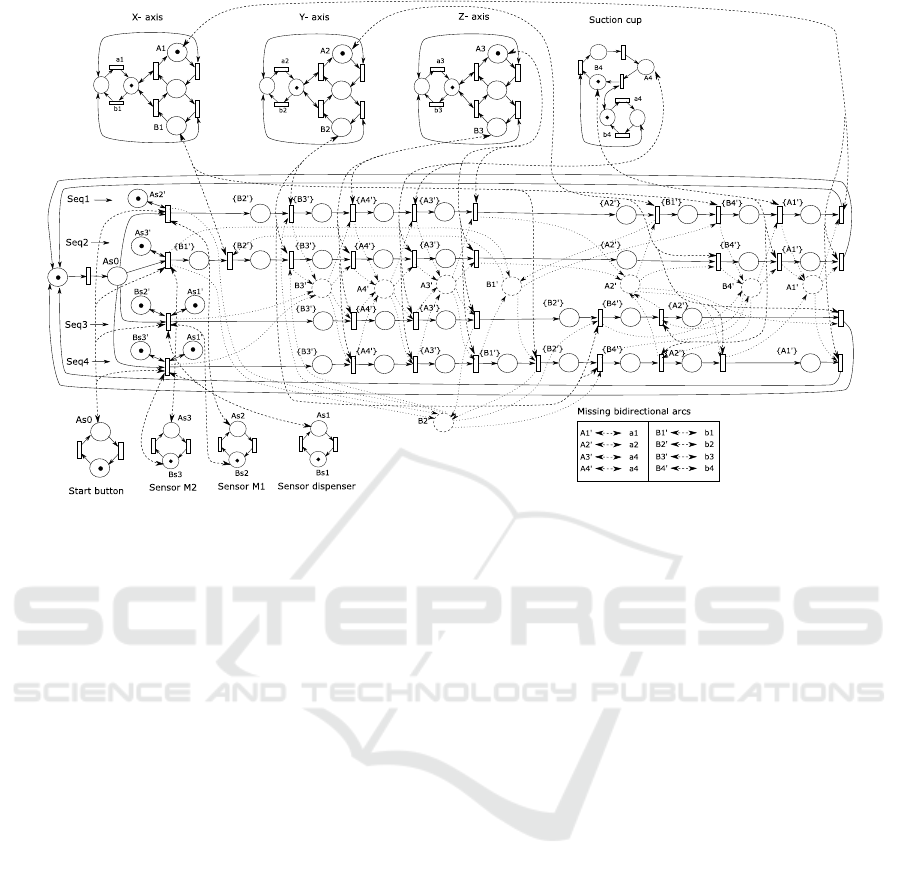
Figure 10: Closed-loop system Q
cl
of the electro-pneumatic arm.
loads M
2
. Qualitatively, every sequence is split into
five subsections: the arm moves to the pic king posi-
tion; the effector (suction cup) turns on; the arm mo-
ves to the placing position; the effector turns off; and
the arm returns to its home position. The initial state
of the arm is its home position.
The specificatio n sequences are the following:
• unloading M
1
and placing the part on the con-
veyor
Seq
1
= B
2
B
3
A
4
A
3
A
2
B
1
B
4
A
1
• unloading M
2
and placing the part on the con-
veyor
Seq
2
= B
1
B
2
B
3
A
4
A
3
A
2
B
4
A
1
• retrieving a part form the dispenser to load M
1
Seq
3
= B
3
A
4
A
3
B
2
B
4
A
2
• retrieving a part form the dispenser to load M
2
Seq
4
= B
3
A
4
A
3
B
1
B
2
B
4
A
2
A
1
The controller is design e d a ccording to the Alg o-
rithm 4.1 presented in subsection 4. Figure 10 pre -
sents the closed loop behavior. The specification is
represented by the nodes in the central area with so-
lid lin e , the four seq uences are indica ted. According
to the proposed controller design methodology, some
guards are added to transitions in sequences: the first
transition of Seq
1
must be g uarded by As2 (i.e. M
1
finished its work), thus the self- loop p la ce As2
′
is ad-
ded to this tr ansition; the first transition of Seq
2
must
be guarded by As3 (i. e., M
2
finished its work), thus
the self-loop place As3
′
is added to this transition; the
first transition of Seq
3
must be guarded by Bs2 (i.e. ,
M
1
is idle), thus the self-loo p place Bs2
′
is added to
this transition; and the first transition of Seq
4
must be
guarde d by Bs3 (i. e., M
4
is idle), thus the self-loop
place Bs3
′
is added to this transition. In addition, the
last two sequences are guarded also by As1, requiring
that a par t is available in the dispenser. The starting
of the four sequences is guarded by As0 , the signal of
the start lock-button.
In Figure 10 dashed circles w ith their input and
output arcs are the places added at steps 5-12 of
the Algorithm 4.1 for mirror places with th e same
symbols (symbols in br ackets {•} represent original
symbols that are removed by step 9). Bidirectional
thick dashed arcs represent synchronizations between
plant’s output places and specification’s transitions,
obtained at steps 19-21 of the Algorithm. For clar ity
of pr esentation, the b idirectional arcs between speci-
fication’s output places and controllable plant’s tr an-
sitions ar e no t drawn (computed a s steps 15-18), ho-
wever, those arcs are indicated in the table in Figure
10.
The corresponding controller can be computed by
eliminating from Q
cl
the no des of the p lant that are
not conne c te d to the specification (i.e., all the plant’s
nodes without symbols). Finally, the resulting con-
troller can be tran slated to a Ladder Diagram for its
implementation in a PLC as explained in ( Santoyo
et al., 2001).
Tracking Control of Electro-pneumatic Systems based on Petri Nets
353

6 CONCLUSIONS
In th is work, a tracking control problem for ENS’s
modeled by IPN’s was addressed. The synth esized
controller enforces the plant to track actuator’s out-
put symbol sequences indicated by the specification.
The IPN plant model is formed as a collection of in-
dividual ENS models herein presented, thus its con-
struction is a straightforward process. The specifica-
tion ind ic ates the actuator’s output symbol sequence,
just as the pr actitioners do, hence it is represented as
a simple IPN sequence. The proposed controller is
capable of handling output symbols of p roximity sen-
sors and switch e s as guards to trigger sequences o f ac-
tuators. Moreover, the closed-loop behavior exhibits
important properties, such as liveness and bounde d-
ness. The proposed approach was illustrated through
an app lication example.
As a future work, the synthesis will be extended to
specifications involving concurre ncy. Moreover, de-
centralized approaches will be investigated.
ACKNOWLEDGEMENTS
The research leading to these results has received fun-
ding f rom the Conacyt Program for Education, project
number 288470.
REFERENCES
Basile, F., C ordone, R., and Piroddi, L. (2013). Integra-
ted design of optimal supervisors for the enforcement
of static and behavioral specifications in Petri net mo-
dels. Automatica, 49(11):3432–3439.
Campos-Rodr´ıguez, R., Ram´ırez-Trevino, A., and L´opez-
Mellado, E. (2004). Regulation control of partially
observed discrete event systems. In IEEE Int. Conf.
on Systems, Man and Cybernetics.
Chao, D. (2009). Direct minimal empty siphon computa-
tion using mip. The International Journal of Advance
Manufacturing Technology, 45(3–4):397–405.
Chen, Y. F., Li, Z. W., Khalgui, M., and Mosbahi, O. (2011).
Design of a maximally permissive liveness-enforcing
Petri net supervisor for flexible manufacturing sys-
tems. IEEE Transactions on Automation Science and
Engineering, 8(2):374–393.
David, R. and Alla, H. (2010). Discrete, Continuous, and
Hybrid Petri nets. Springer.
Ezpeleta, J. (1995). A Petri net based deadlock prevention
policy for flexible manufacturing systems. IEEE Tran-
sactions on R obotics and Automation, 11(2):173–184.
Giua, A., DiCesare, F., and Silva, M. (1992). G eneralized
mutual exclusion constraints on nets with uncontrol-
lable transitions. In IEEE Int. Conf. on Systems, Man
and Cybernetics.
Holloway, L., Krongh, B., and Giua, A. (1997). A survey
of petri net methods for controlled discrete event sys-
tems. Discrete Event Dynamic Systems, 9(2):151–190.
Iordache, M. and Antsaklis, P. (2005). A survey on the su-
pervision of Petri nets. In Int. Conf. on Petri nets.
Li, Z. and Liu, D. (2007). A correct minimal siphons ex-
traction algorithm from a maximal unmarked siphon
of a Petri net. International Journal of Production Re-
search, 45(9):2163–2167.
Li, Z ., Wu, N., and Zhou, M. (2012). Deadlock control
for automated manufacturing systems based on Pet ri
nets. a literature review. IEEE Transactions on Sys-
tems, Man and Cybernetics- Part C: Applications and
Reviews, 42(4):437–462.
Li, Z. and Zhou, M. (2008). On siphon computation for
deadlock control in a class of Petri nets. IEEE Tran-
sactions on Systems, Man and Cybernetics, Part A:
Systems and Humans, 38(3):667–679.
Ramadge, R. and Wonham, W. (1987). Supervisory control
of a class of discrete event processes. SIAM Journal
on Control and Optimi zati on, 25(1):206–230.
Ram´ırez-Prado, G., Santoyo, A., Ram´ırez-Trevino, A., and
Begovich, O. (2000). Regulation problem in discrete
event systems using interpreted petri nets. In I EEE
Int. Conf. on Systems, Man and Cybernetics.
Ram´ırez-Trevino, A., Rivera-Rangel, I., and L´opez-
Mellado, E. (2003). Observability of discrete event
systems modeled by interpreted Petri nets. IEEE Tran-
sactions on R obotics and Automation, 19(4):557–565.
S. Wang, C. W., Zhou, M., and Li, Z. (2012). A method to
compute strict minimal siphons in a class of Petri nets
based on loop resource subsets. IEEE Transactions on
Systems, Man and Cybernetics, Part A: Systems and
Humans, 42(1):226–237.
S´anchez-Blanco, F., Ram´ırez-Trevino, A., and Santoyo, A.
(2004). Regulation control in interpreted Petri nets
using trace equivalence. In IEEE Int. Conf. on Sys-
tems, Man and Cybernetics.
Santoyo, A., Jim´enez-Ochoa, I., and Ram´ırez-Trevino, A.
(2001). A complete cycle for controller design in dis-
crete event systems. In IEEE Int. Conf. on Systems,
Man and Cybernetics.
ICINCO 2018 - 15th International Conference on Informatics in Control, Automation and Robotics
354
