Combining Prediction Methods for Hardware Asset Management

Alexander Wurl

, Andreas Falkner

, Alois Haselb

ock

, Alexandra Mazak

2,∗

and Simon Sperl

Siemens AG

Osterreich, Corporate Technology, Vienna, Austria

TU Wien, Business Informatics Group, Vienna, Austria

Keywords:

Predictive Asset Management, Obsolescence Management, Partial Least Squares Regression, Data Analytics.

Abstract:

As wrong estimations in hardware asset management may cause serious cost issues for industrial systems,

a precise and efﬁcient method for asset prediction is required. We present two complementary methods for

forecasting the number of assets needed for systems with long lifetimes: (i) iteratively learning a well-ﬁtted

statistical model from installed systems to predict assets for planned systems, and - using this regression model

- (ii) providing a stochastic model to estimate the number of asset replacements needed in the next years for

existing and planned systems. Both methods were validated by experiments in the domain of rail automation.

1 INTRODUCTION

A crucial task in Hardware Asset Management

is the

prediction of (i) the numbers of assets of various types

for planned systems, and (ii) the numbers of assets in

installed systems needed for replacement, either due

to end of lifetime (preventive maintenance) or due

to failure (corrective maintenance). This is especi-

ally important for companies that develop, engineer,

and sell industrial and infrastructural systems with a

long lifetime (e.g., in the range of decades) like power

plants, factory equipment, or railway interlocking and

safety systems.

Predicting the number of assets for future projects

is important for sales departments to estimate the po-

tential income for the next years and for bid groups

to estimate the expected system costs. Simple linear

regression models achieve only sub-optimal results

when heterogeneous data sources, faulty data ware-

house entries, or non-standard conditions in installed

systems are involved. Therefore, we combine Partial

Least Square Regression with an iterative algorithm

that removes anomalies introduced by non-standard

conditions and faulty data so that the learned model

can provide optimal prediction results for future pro-

jects.

∗

Alexandra Mazak is afﬁliated with the CDL-MINT at TU

Wien.

Please note, that in this article we use the term ”asset” in

the sense of physical components such as hardware modu-

les or computers but not in the sense of ﬁnancial instru-

ments.

Usually, service contracts oblige a vendor to gua-

rantee the functioning of the system for a given time

period with a failure rate or system down-time lower

than a speciﬁed value. This implies that all failing har-

dware assets (and often also those expected to fail in

near future) must be replaced without delay in order

to ensure continuous service. A precise prediction of

the number of asset types needed in the next n years

is essential for the company to calculate service pri-

ces and to fulﬁll the service obligations for replacing

faulty components. Often, such predictions are made

by experts relying on their experiences and instinct,

including a certain safety margin. A more informed

prediction is based on expectation values: Add the

number of assets in existing systems and the expec-

tation values for the numbers of assets for planned

systems to get a basis for calculating the expectation

values of asset replacements. This kind of prediction

is simple, but it cannot provide information about the

conﬁdence interval of the prediction. A prediction far

below the actual need may cause that assets are not

available in time with all the annoying consequences

for the vendor such as penitent fees and a bad repu-

tation. A prediction far beyond the actual need will

bind costs in unnecessary asset stocks. We provide

a predictive model for the asset replacements, taking

into account all necessary data from installed systems,

project predictions and renewal necessities. The re-

sult is a probability function representing not only the

predicted number of assets but also the uncertainty of

the prediction.

Summarizing our approach, in the ﬁrst step, we

Wurl, A., Falkner, A., Haselböck, A., Mazak, A. and Sperl, S.

Combining Prediction Methods for Hardware Asset Management.

DOI: 10.5220/0006859100130023

In Proceedings of the 7th International Conference on Data Science, Technology and Applications (DATA 2018), pages 13-23

ISBN: 978-989-758-318-6

calculate a regression model capable to predict the

number of assets for planned systems. Using this re-

gression model, the second step provides a predictive

model for the number of new assets and asset repla-

cements needed in the next n years for installed and

planned systems.

This paper is organized as follows: Section 2 pre-

sents the asset regression model for computing the as-

sets of a planned system. Section 3 presents the asset

prediction model for estimating the overall number of

assets needed in the next n years, including assets for

planned systems and renewal assets. Section 4 pre-

sents related work and Section 5 concludes the paper.

2 ASSET REGRESSION MODEL

In this section, we present an iterative learning met-

hod for predicting the number of assets of a given type

needed for a planned system. This model is learned

from the relation between feature and asset numbers

in installed systems (in previous projects). Features

are properties of a system or project that can be coun-

ted or measured by domain experts. For instance, in

the domain of rail automation, features are the num-

bers of track switches, of signals of various types, of

railway crossings, etc. In large systems, there are

hundreds of different features and asset types, whe-

reas the number of installed systems may be lower

than hundred. In order to reduce efforts for the pla-

ners of future projects who need to supply the feature

numbers, we need to ﬁnd a minimal subset of features

that still can predict the number of assets of a given

type with sufﬁcient accuracy.

The problem to ﬁnd a model that predicts assets

from a given amount of features relates to multivariate

data analysis (MVA). One method amongst others in

MVA that addresses similar complex settings is Par-

tial Least Squares Regression (PLSR) (Wold et al.,

2001). PLSR is a technique for collinear data that re-

duces the input variables (i.e., the features) to a smal-

ler set of uncorrelated components and performs least

squares regression on these components. This techni-

que is especially useful when features are highly col-

linear, or when the data set reveals more features than

observations (i.e., installed systems in previous pro-

jects). Furthermore, unlike ordinary multiple regres-

sion, PLSR does not suppose that the set of input fe-

atures is resolved from ambiguities in data. Since

PLSR performs least squares regression on compo-

nents instead of original data, the original data can be

measured with ambiguities. This makes the technique

more robust to measurement uncertainty.

The main two reasons why standard linear regres-

sion does not perform well in our setting are the large

number of input variables compared to the number

of observations, and the fact that some observations

(i.e., some previous projects) contain non-standard

data disrupting the learned model.

2.1 Overview of PLSR

Now we give a brief overview of the PLSR approach

(see, e.g., (Wold, 1980)). The input data set is availa-

ble in the form of the following data matrix:

D =







1,1

··· x

1,p

1,1

··· y

1,d

2,1

··· x

2,p

2,1

··· y

2,d

n,1

··· x

n,p

n,1

··· y

n,d







(1)

Each observation i (1 ≤ i ≤ n) in D corresponds to an

existing system and consists of input variable values

i,1

, . . . , x

i,p

(features) and related output variable va-

lues y

i,1

, . . . , y

i,d

(assets). The task is to exploit the co-

variance relationship between input and output varia-

bles, to estimate the assets for planned systems where

only the features are known. PLSR takes into account

the underlying relationship, i.e., the latent structure,

of features and assets. The matrices X and Y are de-

composed into latent structures in an iterative process.

The latent structure corresponding to the most varia-

tion of Y is extracted and explained by a latent struc-

ture of X that explains it the best.

The model of the population of D consists of

a p-dimensional input variable vector X and a d-

dimensional output variable vector Y. Instead of cal-

culating the parameters β in the linear model

= x

β + ε

in PLSR, we estimate the parameters γ in the so-called

latent variable model

= t

γ + ε

(2)

where the new coefﬁcients γ are of dimension q ≤ p,

ε is an error (noise) term, i.e., the residuals, and the

values t

of the variables are put together in a (n × q)

score matrix T . According to (Wold, 1980), the ob-

jective of PLSR is to estimate the scores T . Due to the

dimension reduction, the regression of y on T should

be more stable. The construction of T is sequentially

performed for k = 1, 2, . . . , q through the PLS criteria

= argmax

Cov(y, Xa)

under the constraints ka

k = 1 and Cov(Xa

, Xa

) = 0

for 1 ≤ j < k. The vectors a

with k = 1, 2, . . . , q are

called loadings, and they are collected in the columns

of the matrix A. The resulting score matrix is then

T = XA.

DATA 2018 - 7th International Conference on Data Science, Technology and Applications

Once the loadings are computed, the regression model

of (2) can be used as predictive regression model for

assets.

2.2 Application of PLSR

One of the major challenges in our problem domain

comes from potential outliers of asset quantities in

the data set. Since the input data originate from he-

terogeneous data sources, anomalies may occur due

to the complexity of merging data structures and due

to non-standard conditions in some projects. Even if

high data quality during the process of data integra-

tion is achieved by approaches such as described in

(Wurl et al., 2017), anomaly detection including mo-

del validation is required during the training phase of

the prediction model.

In model validation, the most common methods

for training regression models are Cross-Validation

(CV) and Bootstrapping. In our setting, CV is pre-

ferred because it tends to be less biased than Boots-

trapping when selecting the model and it provides a

realistic measurement of the prediction accuracy.

To ensure a stable prediction model, we make use

of a double cross-validation strategy which is a pro-

cess of two nested cross-validation loops. The inner

loop is responsible for validating a stable prediction

model, the outer loop measures the performance of

prediction. This strategy is applied to similar approa-

ches that have been described for optimizing the com-

plexity of regression models in chemometrics (Filz-

moser et al., 2009), for a binary classiﬁcation problem

in proteomics (Smit et al., 2008), and for a discrimi-

nation of human sweat samples (Dixon et al., 2007).

Our approach is a formal, partly new combination of

known procedures and methods, and has been imple-

mented in a function for the programming environ-

ment R

, as illustrated in Figure 1.

In the internal cross-validation loop CV1, we train

our model with 80% of the data, using 10-fold cross-

validation. In the external cross-validation CV2, we

test our trained model with the 20% rest of the full

data set.

2.2.1 Training

Our regression model potentially uses all input vari-

ables of all observations to predict a selected output

variable. For each row i = 1..n of the training set as

subset of data matrix D (see Equation 1), the asset a

(a ∈ {1 . . . q}) is estimated by a function f

on the in-

put variables. The predicted values

ˆy

i,a

= f

i,1

, x

i,2

, . . . , x

i,d

)

www.r-project.org

Figure 1: Double Cross-Validation: First, learn a model on

training data set CV1. Second, test the model with the opti-

mal number of components c

opt

on test data set CV2.

should be as close as possible to the real asset values.

”As close as possible” is achieved by an iterative pro-

cess of improving the prediction model step by step,

which is computed by means of PLSR in combination

with CV.

In the inner CV loop, we employ 10-fold CV

to train the model. By training, we aim at ﬁnding

the number of components which adequately explains

both predictors and response variances. This is calcu-

lated by the Root Mean Squared Error of Prediction

(RMSEP) for asset a:

RMSEP =

∑

i=1

i,a

− ˆy

i,a

)

| {z }

quadratic error

The differences y

i,a

− ˆy

i,a

are called residuals. RM-

SEP calculates the residual variation as a function of

the number of components. The result presents for

each component the estimated cross validation error

and the cumulative percentage of variance explained.

Aiming for an optimal number of components, the

goal is to ﬁnd the component with the lowest cross

validation error. The minimum indicates the number

of components with minimal prediction error and an

optimum rank of the cumulative percentage of vari-

ance explained.

While calculating RMSEP, the estimated CV error

usually decreases with an increasing number of com-

ponents. In case of an error increase, it is likely that:

1. Dependent and independent variables are not line-

arly related enough to each other.

2. The data set contains insufﬁcient number of ob-

servations to reveal the relationship between input

and output variables.

Combining Prediction Methods for Hardware Asset Management

3. There is only one component needed to model the

data.

In the outer loop, in addition to RMSEP we use

the signiﬁcance indicator R

. R

is deﬁned by

= 1 −

∑

i,a

− ˆy

i,a

)

∑

i,a

− y

)

(3)

is a value between 0 and 1 and measures how close

the test data are to the values predicted by the regres-

sion model. A low R

value (e.g., R

< 0.9) indicates

that there are still outliers in the observations we used

for training the model. These outliers in the data de-

graded the quality of our model, so we remove them

and train a new model without them.

Algorithm 1 sketches the iterative process of trai-

ning a model for asset prediction. Firstly, the data set

is shufﬂed to obtain a fair distribution of observations.

Secondly, a PLSR regression model is trained and

validated through RMSEP. As a result, the model is

trained again with the optimal number of components

opt

. Thirdly, this model is applied to the test data set

and R

is computed. We use two criteria to decide

whether our model is already good enough or not:

(i) the RMSEP must monotonically decrease with the

number of components used, and (ii) according to lon-

gitudinal studies R

must be at least 0.9 (Mooi et al.,

2018). If the model is not yet good enough, we re-

move all observations from the data set that we cate-

gorized as outliers. After some experiments, the follo-

wing outlier classiﬁcation has turned out to be useful:

Outliers are observations with residuals that are larger

than 25% of the maximum asset value in the data set.

After removing the noisy observations, learning starts

again. We proceed with this learning cycle until our

model meets the above mentioned quality criteria or

no improvement could be achieved.

In the last step of Algorithm 1, the features that

signiﬁcantly contribute to a prediction are extracted

according to their weights. Currently, this selection is

done by a domain expert based on the weights of the

features that dominate the prediction model.

2.3 Prediction

Our trained model is now

ˆy

= f

) (4)

where X

⊆ {x

, . . . , x

} is the set of signiﬁcant fea-

tures used for predicting assets of type a based on a

Algorithm 1: Calculate Asset Regression Model.

1. Shufﬂe rows in the data set to obtain a fair dis-

tribution of observations.

2. Train a PSLR regression model

(a) Apply a 10-fold cross-validation to the trai-

ning data set.

(b) Compute RMSEP and evaluate optimal

numbers of components c

opt

ning data set using c

opt

3. Test model on test data set by computing R

If RMSEP does not monotonically decrease

with the number of components,

or if R

< 0.9

(a) Identify outliers in observations and remove

them.

(b) Go to step 2.

4. Extract signiﬁcant features to select the ﬁnal

prediction model.

model f

. Applying this model to concrete feature

values

of features X

for a planned system will

provide an expectation value for the number of as-

sets a. In this sense, the output variable ˆy

could be

seen as a random variable with a normal distribution

- ˆy

∼ N (µ, σ

) - where the mean value µ is f

(

)

and σ is the above described mean square error RM-

SEP. Therefore, a 95% conﬁdence interval is given by

= ˆy

± 2 ∗ RMSEP (Friedman et al., 2001). In the

next subsection, we demonstrate this on an example.

2.4 Example and Experimental Results

We tested validity of our method on a data set from the

railway safety domain with data collected over about

a decade. Our data set contained ca. 140 features

(input variables), ca. 300 assets (potential output va-

riables), and ca. 70 observations (installed systems).

We chose the concrete asset type A41 - a hardware

module that controls track switches - to demonstrate

training of the regression model and prediction. We

implemented this example and the regression training

algorithm in R, making use of the plsr() function in

the pls library

Before starting any calculation, we preprocessed

the data set by removing all assets except A41 and

shufﬂed the data set in order to have a fair distribution

of the training data set and the test data set. Following

Algorithm 1, we built the model by specifying A41 as

the output variable and all features as input variables,

and performed 10-fold cross-validation based on the

NIPALS algorithm (Wold, 1966; Wold, 1980).

http://mevik.net/work/software/pls.html

DATA 2018 - 7th International Conference on Data Science, Technology and Applications

0 20 40

100

measured

predicted

(a) Cycle 1: RMSEP=14.11, R

=0.35

0 20 40

100

measured

predicted

(b) Cycle 2: RMSEP=2.77, R

=0.87

0 20 40

100

measured

predicted

=0.94

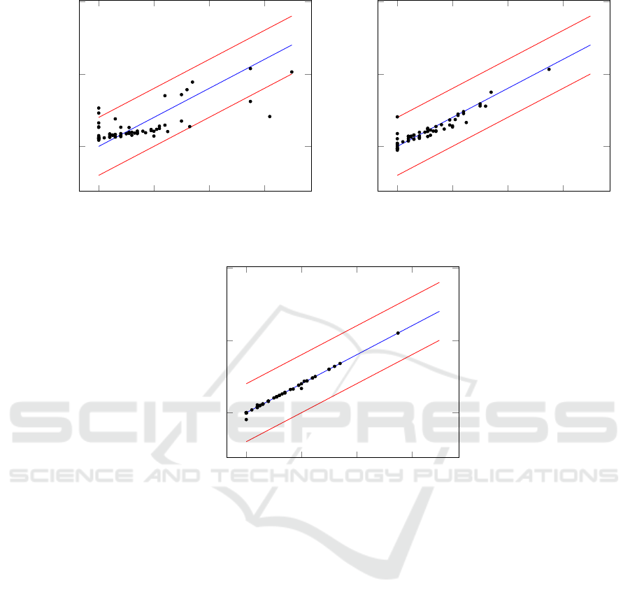
Figure 2: Three cycles for training a regression model for asset A41.

Figure 2 shows the three training cycles for A41.

After the ﬁrst cycle, four observations were identiﬁed

as outliers and removed from the training set. After

the second cycle, another two observations were re-

moved. After the third cycle we ended up in a regres-

sion model of high precision.

The features are the input variables of the regres-

sion model. Their values must be provided by domain

experts. To compute/count/measure these feature va-

lues (e.g., counting the signals of various types in a

railway station, or measuring the distances between

signals on the tracks) is often a time-consuming and

expensive task. The reduction of the feature set to a

small subset of signiﬁcant ones with satisfying pre-

dictive power will save time and costs, especially in

the usually very stressful phase of proposal prepara-

tion.

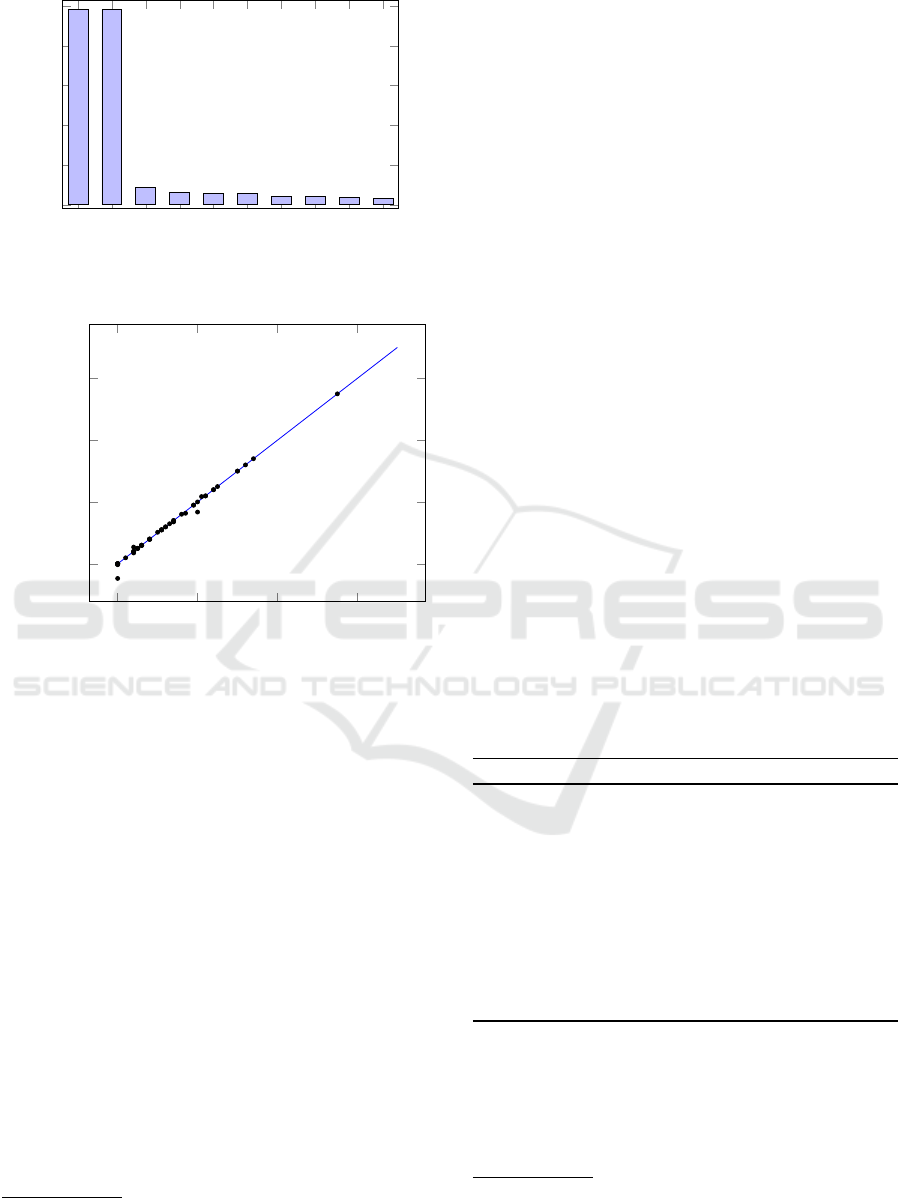
Therefore we identiﬁed the most signiﬁcant input

variables by analyzing the coefﬁcients of the input va-

riables in the model. Figure 3 shows the ﬁrst 10 posi-

tive coefﬁcients sorted by their values. It can easily be

seen that feature F31 (corresponding to the number of

track switches of the railway station) and feature F32

(corresponding to the number of track key-locks) have

much more impact on asset A41 than all the other fe-

atures. We learned a ﬁnal model based on these two

input variables only. This ﬁnal model, as shown in

Figure 4, is used for predicting the asset values in the

test data set and does not show noticeable differences

to the results of the last iteration (see Figure 2 (c)),

although it is based on two features only.

We tested the described method on other asset ty-

pes, e.g. on hardware modules for controlling track-

side signals, and it shows a similar behavior – after a

few cycles of outlier removal the learned regression

models have high prediction quality.

Combining Prediction Methods for Hardware Asset Management

F31

F32

F14

F22

F94

F42

F111

0.2

0.4

0.6

0.8

Features

Figure 3: Importance Analysis of Features.

0 20 40

measured

predicted

Figure 4: Final linear regression model for asset A41 based

on features F31 and F32 only.

3 ASSET PREDICTION MODEL

Building upon the regression model of the previous

section, in this section we present a stochastic model

for answering the following question: How many as-

sets of type A are needed in the next n years? The

input parameters of this problem are:

• An asset type A. Associated with an asset type is

a failure rate, like MTBF (mean time between fai-

lure). MTBF is the expected time between failures

of the asset. We only consider failures that cause

the replacement of the asset.

The failures can be

seen as random samples of a non-repairable popu-

lation and the failure times follow a distribution

with some probability density function (PDF).

• A scope S = {s

, . . . , s

} is a set of asset groups.

Basically, each asset group corresponds to all as-

sets of type A of an installed or planned system

A detailed differentiation of MTBF and MTTF (Mean

Time To Failure) is beyond the scope of this paper.

that must be taken into account for the forecast.

Each member of an asset group must have the

same installation date. As we will see later, this is

important for computing the renewal numbers (ol-

der assets are more likely to fail than newer ones).

Therefore, an installed system may be represen-

ted by more than one asset group: one group for

all assets initially installed and still alive, and the

other groups for the already necessary asset repla-

cements.

Each s ∈ S has the following properties:

– M

is a random variable representing the num-

ber of assets in the asset group s ∈ S; Pr(M

n), n ∈ N, is the probability that s contains n

elements.

– tbos

: Begin of service time of all assets in s ∈

S. At this point in time the assets has been or

will be installed in the ﬁeld.

– teos

: End of service time of all assets in s ∈

S. This is the time where the service contract

ends. After this point in time the assets need no

longer be replaced when failed.

– A probability q

∈ [0, 1] representing the like-

lihood that the system containing s ∈ S will be

ordered. Trivially, for already installed assets

= 1.

• A point in time t

target

∈ N up till that the prediction

should be made. All assets in the scope whose

service times overlap the period [t

now

target

] are to

be taken into account. The service time of interest

for each asset group s ∈ S is then

= min(teos

target

) −tbos

Algorithm 2: Total Asset Prediction.

1. Input: (i) asset type A (ii) scope (iii) target time

target

2. Collect asset groups of given asset type and gi-

ven scope: S = {s

, . . . , s

}

(a) Existing assets from installed systems

(b) Asset predictions for planned systems

3. Perform renewal asset analysis:

4. Compute estimator for each asset group:

5. Sum up asset group estimators:

total

∑

s∈S

Please note that the computation of the forecast

model is always done for assets of a given type A, so

for the sake of simplifying the notation we omit to

subscript all variables with A in this section.

The prediction of needed assets must take into ac-

count both renewal of already installed assets in case

We use a simple representation of time: years started from

some absolute zero time point. This simpliﬁes arithmetic

operations on time variables.

DATA 2018 - 7th International Conference on Data Science, Technology and Applications

of non-repairable failures and new assets needed for

planned systems. We will present a stochastic model

that combines both cases. Algorithm 2 summarizes

the steps how to compute such a prediction model. In

step 1, the user has to provide an asset type, a scope,

and a target point in time. In step 2, the asset groups

from the installed base (existing projects) and the sa-

les database (future projects) are collected. Then a

stochastic model that represents needed renewal as-

sets is computed based on failure rates/failure distri-

butions of the assets and the service time periods of

the asset groups. In step 4, an estimator is computed

for each asset group using project order probability,

the probability of the number of assets in the group,

and the renewal model. Finally, all these estimators

are summed up to an overall asset estimator

total

We present the details in the next subsections.

3.1 Renewal Processes

To estimate the number of assets needed for replace-

ment of failing assets we resort to the theory of re-

newal processes, see, e.g., (Grimmett and Stirzaker,

2001; Randomservices.org, 2017). In this subsection,

we recap the main deﬁnitions of renewal processes

and show how we apply it to predict the number of

assets that must be replaced because of failures. A re-

newal process is a stochastic model for renewal events

that occur randomly in time. Let X

be the random

variable representing the time between 0 and the ﬁrst

necessary renewal of an asset. The random variables

, X

, . . . are the subsequent renewals. These varia-

bles X

are called inter-arrival times. In our case, their

distribution is directly connected to the failure rates

or MTBF of the asset type. So (X

, X

, . . .) is a se-

quence of independent, identically distributed random

variables representing the time periods between rene-

wals. X

takes values from [0, ∞), and Pr(X

> 0) > 0.

Let f

(t) be the PDF and F

(t) = Pr(X ≤ t) be the

distribution function of the variables X

The random variable T

for some number n ∈ N

represents the so-called arrival time; F

(t) = Pr(T

≤

t) represents the probability of n renewals up to time

t. T

is simply the sum of the inter-arrival variables

∑

i=1

The PDF of T

is therefore the convolution of its con-

stituents:

= f

∗n

= f

∗ f

∗ . . . ∗ f

Remark. To add two random variables one has to

apply the convolution operator on the their PDFs. The

convolution operator ∗ for two functions f and g is

deﬁned as

( f ∗ g)(t) =

f (t

)g(t − t

)dt

, continuous case

( f ∗ g)(n) =

∞

∑

m=−∞

f (m)g(n − m) , discrete case

The expression f

∗n

stands for applying the convo-

lution operator on a function f n times. For many

probability distribution families, summing up two

random variables and therefore computing the con-

volution of their PDFs is easy. For instance, the sum

of two Poisson distributed variables with parameters

and λ

is: Poi[λ

] + Poi[λ

] = Poi[λ

+ λ2]. (End

of remark.)

In the renewal process, the arrival time variables

are used to create a random variable N

that counts

the number of expected renewals in the time period

[0,t]. It is deﬁned in the following way:

= |{n ∈ N : T

≤ t}| for t ≥ 0

The arrival time process T

and the counting pro-

cess N

are kind of inverse to each other, where the

probability distribution of N

can be derived from the

probability distribution of T

. Thus, the theory of re-

newal processes gives us a tool for deriving the coun-

ting variable N

from a given failure distribution X

of an asset. For complicated distributions of X, the

derivation of N

could get elaborate and could rea-

sonably be done by numeric methods only, but it is

straight-forward for some prominent distribution fa-

milies. The most important case is the Poisson pro-

cess, where X has an exponential distribution with pa-

rameter λ. In this case, the n-th arrival time variable

has a Gamma distribution with shape parameter n

and rate parameter λ, and the counting variable N

has

a Poisson distribution with parameter λt.

3.2 Prediction Model

In this subsection we describe how to combine the

number of assets in each asset group M

(s ∈ S), the

above described renewal counting variable N

, and

the probability q

representing the likelihood that the

assets will be ordered to an estimator, i.e., a proba-

bility mass function

(PMF), reﬂecting the number of

needed assets in a given time period.

Deﬁnition 1 (Renewal Estimator

). Let M

be a

random variable representing the number of assets in

the asset group s ∈ S. Let N

be the renewal coun-

ter for the service time period τ

of asset group s.The

renewal estimator

is a random variable, where

A probability mass function (PMF) is the discrete counter-

part of a probability distribution function (PDF). A PMF

f (n) corresponding to a random variable X is Pr(X =

n), n ∈ N.

Combining Prediction Methods for Hardware Asset Management

Pr(

= n), n ∈ N, is the probability that exactly n

renewal assets are needed in total for the asset group

s ∈ S. It’s PMF f

is deﬁned in the following way:

(n) :=

∞

∑

k=0

(k) f

∗k

(n) (5)

Deﬁnition 2 (Asset Group Estimator

). Let M

a random variable representing the number of assets

in the asset group s ∈ S. Let q

be the probability

that the project containing the assets of s are orde-

red at all. Let

be the renewal estimator as deﬁned

above.

is a random variable with Pr(

= n), n ∈ N,

representing the probability that the number of assets

needed for s is exactly n. It is the sum of the number of

assets and the number of renewals scaled by the order

probability. Its PMF is:

(n) := q

( f

(n) ∗ f

(n)) + (1 − q

)δ

(n) (6)

Remark. The delta function δ

(x) (also called unit

impulse) is 1 at x = k and otherwise 0. We use the

delta function here to express certainty of zero assets

in the case that the project will not be ordered. As we

use later, the convolution with the delta function can

be used for shifting: f (x) ∗ δ

(x) = f (x − k). (End of

remark.)

Deﬁnition 3 (Total Asset Estimator

total

). The to-

tal asset estimator

total

is a random variable with

Pr(

total

= n),n ∈ N, representing the probability that

the total number of assets needed for all asset groups

s ∈ S until t

target

is exactly n. It is the sum of the asset

group estimators

total

∑

s∈S

(7)

Its PMF is the convolution of the PMFs of the asset

group estimators

total

(n) :=

∗

s∈S

(n) (8)

The probability distribution f

total

can now be

used for calculating its expectation value, its variance

or standard deviation, but also the number of needed

assets with a guaranteed probability that the number

will be high enough, i.e., compute the smallest n with

Pr(

total

<= n) is greater or equal some given pro-

bability, like 0.75 or 0.95, depending on the certainty

the forecast should provide.

The design of the variables in this framework is

both suited for installed and planned systems. For a

planned system, the probability that the system will be

ordered is an information provided by sales experts.

The estimation of how many assets will be needed

can be predicted by the regression model described in

Section 2. In this case, the estimator M

corresponds

to a random variable derived from the regression mo-

del ˆy = f ( ¯x), where ¯x is the feature vector of the plan-

ned system. See Equation 4 in Section 2.3.

For asset groups of installed systems, the order

probability q

is simply 1, and the estimator variable

for the asset count is the delta function δ

(n) with

k being the actual number of installed assets. In this

case the asset group estimator

is simply the shifted

renewal estimator

with PDF f

(n − k). It should

be noted that

total

not only contains predicted assets,

but also all already installed assets. These could be

simply subtracted from

total

, if only the number of

assets to be ordered in the future are needed.

3.3 Example

Figure 5 shows a small example that shall demon-

strate the combination of statistical methods of our

asset prediction framework.

Figure 5: Example of an asset prediction problem, contai-

ning 3 asset groups of existing projects (s

, s

) and 2 fu-

ture projects with asset groups s

and s

We use an exponential distribution of the failure

rates of the assets with λ = 0.125 (i.e., 0.125 failu-

res per year expected), corresponding to a MTBF of 8

years. So the renewal counting variables N

are Pois-

son distributed: N

∼ Poi(λτ). The number of assets

of the existing systems 1 to 3 are 6, 4, and 15, so

∼ δ

, M

∼ δ

, and M

∼ δ

. The number es-

timators M

and M

of the two planned systems are:

: Pr(M = 7) = 0.2, Pr(M = 8) = 0.6, Pr(M = 9) =

0.2; M

: Pr(M = 8) = 0.05, Pr(M = 9) = 0.1, Pr(M =

10) = 0.7, Pr(M=11)=0.1, Pr(M = 12) = 0.05. The

resulting asset group estimators and the total asset

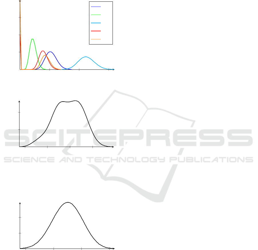
estimator are depicted in Fig. 6. Some interesting

results are shown in Table 1. The ﬁrst row shows

the resulting expectation values of the number of as-

sets. The other rows in Table 1 show the variances

and standard deviations of our estimator probability

functions, along with 3 examples of asset estimati-

ons with speciﬁed likelihood, i.e., F

−1

(p) stands for

the number of assets n with Pr(F ≤ n) >= p. While

usually only this expectation value is used for asset

DATA 2018 - 7th International Conference on Data Science, Technology and Applications

prediction, our approach provides valuable additional

information, like the standard deviation, and the pos-

sibility to ﬁnd an asset number estimation with high

reliability, like F

−1

(0.95).

20 40

0.100

0.200

0.300

0.400

(n)

(a) Asset Group Estimators

80 100 120

0.010

0.020

total

(n)

(b) Total Asset Estimator

total

Figure 6: Probability mass functions of predicted assets for

asset groups and total asset estimator for the example sce-

nario depicted in Fig. 5.

900

950

1,000

1,050

0.005

0.010

total

(n)

Figure 7: Probability mass function for an estimator of asset

A41. 580 assets are already installed. The total expectation

value

is 975 (corresponds to 395 new assets), the standard

deviation σ is 26.30, F

−1

(0.75) = 993 (corresponds to 413

new assets), F

−1

(0.95) = 1018 (corresponds to 438 new

assets).

Figure 7 shows the resulting total asset estimator

of a real world example. We applied our method to the

data set used in Section 2.4 and computed a predictor

for the number of assets of type A41 for the next 10

years. About 40 installed systems with 580 instances

of asset A41 and 7 future systems have been taken into

account. Subtracting the already installed 580 assets,

we get an expectation value of 395 additional assets,

covering the assets for the 7 new systems and asset

renewals. A prediction with 95% likelihood results in

438 new assets.

4 RELATED WORK

In industry, asset management is deﬁned as the ma-

nagement of physical, as opposed to ﬁnancial, assets

(Amadi-Echendu et al., 2010). Managing assets may

comprise a broad range of different potentially over-

lapping objectives such as planning, manufacturing,

and service. Depending on the scope of asset mana-

gement, the data included determine the possibilities

of predictive data analytics (Li et al., 2015). An es-

sential part of asset management, especially in manu-

facturing, is to estimate the condition (health) of an

asset.

In the last decade, an engineering discipline, cal-

led prognostics, has evolved aiming to predict the re-

maining useful life (RUL), i.e., the time at which a

system or a component (asset) will no longer per-

form its intended function (Vachtsevanos et al., 2006).

Since the reason for non-performance is most often a

failure, data-driven prognostics approaches consist of

modeling the health of assets and learning the RUL

from available data (Mosallam et al., 2015; Mosallam

et al., 2016). (Bagheri et al., 2015) present a stochas-

tic method for data-driven RUL prediction of a com-

plex engineering system. Based on the health value of

assets, logistic regression and the assessment output is

used in a Monte Carlo simulation to estimate the re-

maining useful life of the desired system. (Lee et al.,

2017) calculate the weighted RUL of assets to op-

timize the productivity in cyber-physical manufactu-

ring system by applying Principal Component Analy-

sis (PCA) in combination with Restricted Boltzmann

Machine (RBM).

Other predictive methods aim for predicting the

obsolescence of assets based on sales data. (Sandborn

et al., 2007) propose a data-mining approach inclu-

ding linear regression to estimate when an asset beco-

mes obsolete. Based on this approach, (Ma and Kim,

2017) use time series models instead of linear regres-

sion models and state that prediction over years may

be inaccurate. (Jenab et al., 2014) examine the de-

tection of obsolescence in a railway signaling system

with a Markovian model and mention that forecasting

obsolescence of assets may be inexact. (Thaduri et al.,

Combining Prediction Methods for Hardware Asset Management

Table 1: Some resulting probability values for the example scenario depicted in Fig. 5.

Total

21 9 45 13 11 99

var 14.91 4.97 29.68 47.95 78.47 175.58

σ 3.86 2.23 5.45 6.92 8.86 13.25

−1

(0.50) 21 9 45 15 15 99

−1

(0.75) 24 10 49 17 18 108

−1

(0.95) 28 13 54 21 22 119

2015) draft the potential application of predictive as-

set management in the railway domain by incorpora-

ting heterogeneous data sources such as construction

and sales data. One of the main challenges is pre-

dictive asset management for long-term maintenance

which coincides with our context.

One possible starting point to address the pre-

diction of long-term asset management is formulating

the product life cycle with evolutionary parametric

drivers that describe an asset type whose performance

or characteristics evolve over time (Solomon et al.,

2000). Since evolutionary parametric drivers cannot

be found in our database, procurement life modeling

may be used (Sandborn et al., 2011). The most pro-

minent model of the mean procurement life, which

is analogous to the mean-time-to-failure (MTTF), is

the bathtub curve (Klutke et al., 2003), usually mo-

deled by Weibull distributions. This model represents

three regimes in the lifetime of a hardware module:

the ﬁrst phase shows high but decreasing failure ra-

tes (”infant mortality”), the main, middle phase shows

low, constant failure rates, and the third phase repre-

sents ”wear out failures” and therefore increasing fai-

lure rates.

A prominent model in preventive maintenance

(see, e.g., (Gertsbakh, 2013)) represents the replace-

ment of an asset after a constant time before the fai-

lure probability gets too high. This can be modeled by

a distribution function F that consists of two parts: the

ﬁrst part is some ”conventional” distribution function,

but from a deﬁned replacement time t

on, the proba-

bility of replacement is just 1.

Our input data is taken from the installed base (da-

tabase of currently installed systems) and the sales da-

tabase containing forecasts of expected future projects

(planned systems). Unlike previous predictive obso-

lescence approaches where the main goal is to esti-

mate the date when particular assets become obsolete,

the combination of our data sets enables us to repre-

sent not only the numbers of renewal assets needed

for n years but also the uncertainty of the estimation

for long-term maintenance.

5 CONCLUSION AND FUTURE

WORK

In this paper, we proposed a predictive asset manage-

ment method for hardware assets. The proposed met-

hod consists of two phases: In the ﬁrst phase, a regres-

sion model is learned from installed systems to pre-

dict assets for planned systems. In the second phase,

a stochastic model is used for summing up all assets

needed in the next n years for existing and also future

projects, taking renewals of failing components into

account. In experiments we validated our method in

the domain of railway safety systems.

There are several ideas for future work: Currently,

when calculating an asset regression model we ap-

ply PLSR in an iterative way. In future work, we

aim at a broader evaluation by comparing additional

methods such as Sparse partial robust M-regression

(Hoffmann et al., 2015), or Robust and sparse estima-

tion methods for high dimensional linear and logistic

regression (Kurnaz et al., 2017).

In our approach we train the model for each asset

type separately. This means that the set of features

for each regression model is minimized for each asset

separately. An important problem for future work is

to ﬁnd a minimal subset of features that is signiﬁcant

for predicting all assets. Furthermore, it would be in-

teresting to take costs of feature measurement into ac-

count. E.g., in the railway domain it is easier to count

signals and track switches than insulated rail joints of

a railroad region. An optimal subset of features is one

with minimal total measurement costs.

Presently, we use a given MTBF per asset type

in our method. We assume that prediction accuracy

can be further improved by applying advanced prog-

nostics techniques for customizing the MTBF to the

respective system context.

Although we tested our method only on data from

rail automation, we suppose that applying it to har-

dware components in other domains will produce si-

milar results of prediction. This needs to be evaluated

in future work.

DATA 2018 - 7th International Conference on Data Science, Technology and Applications

ACKNOWLEDGEMENTS

This work is funded by the Austrian Research Promo-

tion Agency (FFG) under grant 852658 (CODA). We

thank Walter Obenaus (Siemens Rail Automation) for

supplying us with test data.

REFERENCES

Amadi-Echendu, J. E., Willett, R., Brown, K., Hope, T.,

Lee, J., Mathew, J., Vyas, N., and Yang, B.-S. (2010).

What Is Engineering Asset Management?, pages 3–

16. Springer London, London.

Bagheri, B., Siegel, D., Zhao, W., and Lee, J. (2015).

A Stochastic Asset Life Prediction Method for

Large Fleet Datasets in Big Data Environment. In

ASME 2015 International Mechanical Engineering

Congress and Exposition, pages V014T06A010–

V014T06A010. American Society of Mechanical En-

gineers.

Dixon, S. J., Xu, Y., Brereton, R. G., Soini, H. A., Novotny,

M. V., Oberzaucher, E., Grammer, K., and Penn, D. J.

(2007). Pattern recognition of gas chromatography

mass spectrometry of human volatiles in sweat to dis-

tinguish the sex of subjects and determine potential

discriminatory marker peaks. Chemometrics and In-

telligent Laboratory Systems, 87(2):161–172.

Filzmoser, P., Liebmann, B., and Varmuza, K. (2009). Re-

peated double cross validation. Journal of Chemome-

trics, 23(4):160–171.

Friedman, J., Hastie, T., and Tibshirani, R. (2001). The

elements of statistical learning, volume 1. Springer

series in statistics New York.

Gertsbakh, I. (2013). Reliability theory: with applications

to preventive maintenance. Springer.

Grimmett, G. and Stirzaker, D. (2001). Probability and

random processes. Oxford university press.

Hoffmann, I., Serneels, S., Filzmoser, P., and Croux, C.

(2015). Sparse partial robust M regression. Chemome-

trics and Intelligent Laboratory Systems, 149:50–59.

Jenab, K., Noori, K., and Weinsier, P. D. (2014). Obsoles-

cence management in rail signalling systems: concept

and markovian modelling. International Journal of

Productivity and Quality Management, 14(1):21–35.

Klutke, G., Kiessler, P. C., and Wortman, M. A. (2003). A

critical look at the bathtub curve. IEEE Trans. Relia-

bility, 52(1):125–129.

Kurnaz, F. S., Hoffmann, I., and Filzmoser, P. (2017).

Robust and sparse estimation methods for high-

dimensional linear and logistic regression. Chemome-

trics and Intelligent Laboratory Systems.

Lee, J., Jin, C., and Bagheri, B. (2017). Cyber physical

systems for predictive production systems. Production

Engineering, 11(2):155–165.

Li, J., Tao, F., Cheng, Y., and Zhao, L. (2015). Big data

in product lifecycle management. The Internatio-

nal Journal of Advanced Manufacturing Technology,

81(1-4):667–684.

Ma, J. and Kim, N. (2017). Electronic part obsolescence fo-

recasting based on time series modeling. International

Journal of Precision Engineering and Manufacturing,

18(5):771–777.

Mooi, E., Sarstedt, M., and Mooi-Reci, I. (2018). Market

Research. Springer.

Mosallam, A., Medjaher, K., and Zerhouni, N. (2015).

Component based data-driven prognostics for com-

plex systems: Methodology and applications. In Re-

liability Systems Engineering (ICRSE), 2015 First In-

ternational Conference on, pages 1–7. IEEE.

Mosallam, A., Medjaher, K., and Zerhouni, N. (2016).

Data-driven prognostic method based on bayesian ap-

proaches for direct remaining useful life prediction.

Journal of Intelligent Manufacturing, 27(5):1037–

1048.

Randomservices.org (2017). Renewal processes. http://

www.randomservices.org/random/renewal/index.html

[Online; accessed 3-February-2018].

Sandborn, P., Prabhakar, V., and Ahmad, O. (2011). Fore-

casting electronic part procurement lifetimes to enable

the management of DMSMS obsolescence. Microe-

lectronics Reliability, 51(2):392–399.

Sandborn, P. A., Mauro, F., and Knox, R. (2007). A data

mining based approach to electronic part obsolescence

forecasting. IEEE Transactions on Components and

Packaging Technologies, 30(3):397–401.

Smit, S., Hoefsloot, H. C., and Smilde, A. K. (2008). Sta-

tistical data processing in clinical proteomics. Journal

of Chromatography B, 866(1-2):77–88.

Solomon, R., Sandborn, P. A., and Pecht, M. G. (2000).

Electronic part life cycle concepts and obsolescence

forecasting. IEEE Transactions on Components and

Packaging Technologies, 23(4):707–717.

Thaduri, A., Galar, D., and Kumar, U. (2015). Railway

assets: A potential domain for big data analytics. Pro-

cedia Computer Science, 53:457–467.

Vachtsevanos, G. J., Lewis, F., Hess, A., and Wu, B. (2006).

Intelligent fault diagnosis and prognosis for engineer-

ing systems. Wiley Online Library.

Wold, H. (1966). Nonlinear Estimation by Iterative Least

Squares Procedures in: David, FN (Hrsg.), Festschrift

for J. Neyman: Research Papers in Statistics, London.

Wold, H. (1980). Model construction and evaluation when

theoretical knowledge is scarce: Theory and applica-

tion of partial least squares. In Evaluation of econo-

metric models, pages 47–74. Elsevier.

Wold, S., Sj

ostr

om, M., and Eriksson, L. (2001). Pls-

regression: a basic tool of chemometrics. Chemo-

metrics and intelligent laboratory systems, 58(2):109–

130.

Wurl, A., Falkner, A., Haselb

ock, A., and Mazak, A.

(2017). Using signiﬁers for data integration in rail

automation. In Proceedings of the 6th International

Conference on Data Science, Technology and Appli-

cations, volume 1, pages 172–179.

Combining Prediction Methods for Hardware Asset Management