
Modeling and Validation of a Complex Vehicle Dynamics Model for
Real-time Applications
Peter Riegl and Andreas Gaull
Carissma, Ingolstadt Univ. of Applied Sciences, Esplanade 10, Ingolstadt, Germany
Keywords:
Vehicle Dynamics, Twin Track Model, Real-time, Tire Model, Magic Formula.
Abstract:
This paper deals with the modeling and validation of a complex vehicle dynamics model implemented in
Matlab, which should enable real-time simulation. In detail, the powertrain and the tire model Magic Formula
by Pacejka are presented. In addition to the horizontal dynamics, which can also be found in single track
models, the here presented vehicle model also takes into account the vertical motion as well as the pitch
and roll behavior. Furthermore, the wheel load fluctuations during the driving maneuvers are included. The
equations of motion are based on multi-body dynamics. Based on three driving scenarios, which are simulated
in the software CarMaker, the quality of the driving dynamics model is evaluated.
1 INTRODUCTION
In addition to the passive safety of a vehicle aimed at
reducing the consequences of a traffic accident, active
vehicle safety has become increasingly important in
recent years. The main goal of active safety systems
is to detect possible dangers in advance with the help
of electronic vehicle control systems and to initiate
countermeasures by means of targeted interventions
on the vehicle motion in order to avoid collisions. An-
other development trend is the autonomous driving.
Here vehicle control systems take over the control of
the vehicle during steering, braking and acceleration
maneuvers, without human intervention being neces-
sary. For this, the current vehicle parameters have to
be known. Furthermore, information about the posi-
tion of the vehicle relative to the road and about other
road users is needed. This data have be identified by
suitable sensors like GPS, cameras or Lidar. Both,
active vehicle safety and autonomous driving require
control algorithms that process the provided sensor
data in real-time and perform corresponding control
interventions. For the development and the testing
of such control systems in critical situations real-time
vehicle dynamics models are necessary, which take
into account all important influences on the vehicle
handling with a sufficient accuracy. This is not always
guaranteed in the case of simplistic models used so
far in many studies like single track models and twin
track models, whose center of gravity is on the road
level. Therefore, it is necessary to develop a nonlinear
twin track model, which also takes into account the
vertical dynamics with the occurring pitch and roll of
the vehicle body. This model should indicate the same
behavior as complex systems like CarMaker that used
for validation.
2 NONLINEAR TWIN TRACK
MODEL
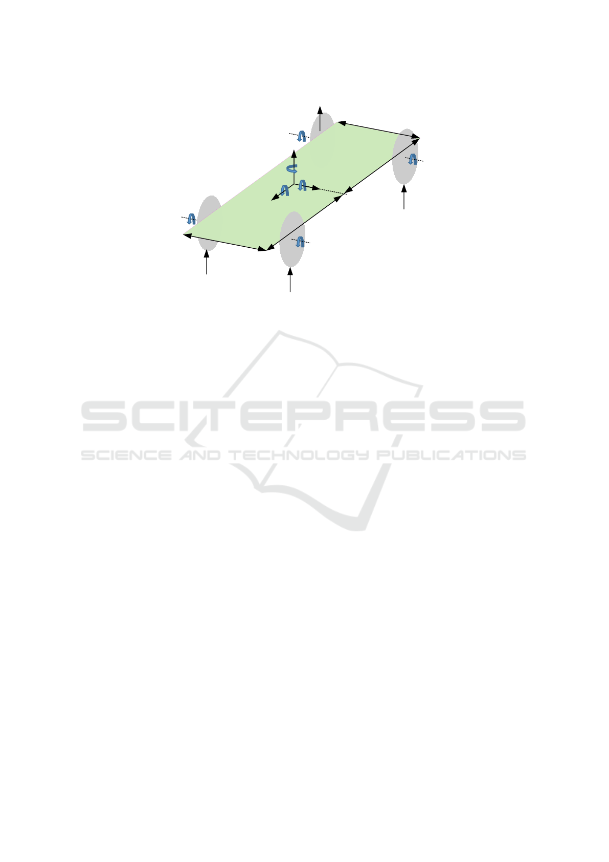
2.1 Kinematics
The kinematics of the vehicle body can be described
by means of three translational x
V
, y
V
, z
V
and three
rotational degrees of freedom ϕ, θ, ψ. Furthermore,
each wheel performs a rotation ρ
j
about its wheel-
carrier-fixed axis. In this paper, the index j indicates
the components front left, front right, rear left or rear
right. The suspension, whose exact kinematics is dis-
regarded here, enables a vertical motion of the wheel.
The tire deflection z
W
j
results from the wheel load
changes and the road bumps. Thus, the vehicle model
has in total 14 degrees of freedom (cf. figure 1). To
describe the equations of motion, the generalized co-
ordinates and generalized velocities are summarized
as state vectors (Schramm et al., 2018):
z
z
z =
h
x
V
, y
V
, z
V
, ϕ, θ, ψ, z
W
f l
, z
W
f r
, z
W
rl
, z
W
rr
,
ρ
f l
, ρ
f r
, ρ
rl
, ρ
rr
i
T
=
h
I
r
r
r
IV
, Φ
Φ
Φ
IV
, z
z
z
W
, ρ
ρ
ρ
i
T
(1)
Riegl, P. and Gaull, A.
Modeling and Validation of a Complex Vehicle Dynamics Model for Real-time Applications.
DOI: 10.5220/0006856304030413
In Proceedings of 8th International Conference on Simulation and Modeling Methodologies, Technologies and Applications (SIMULTECH 2018), pages 403-413
ISBN: 978-989-758-323-0
Copyright © 2018 by SCITEPRESS – Science and Technology Publications, Lda. All rights reserved
403
˙
ρ
rl
˙
ρ
rr
˙
ρ
fl
˙
ρ
fr
z
W
fr
z
W
fl
z
W
rl
z
W
rr
s
r
s
f
l
f
y
V
x
V
z
V
θ
φ
ψ
l
r
Figure 1: Vehicle model.
u
u
u =
h
v
x
, v
y
, v
z
, ω
x
, ω
y
, ω
z
, ˙z
W
f l
, ˙z
W
f r
, ˙z
W
rl
, ˙z
W
rr
,
˙
ρ
f l
,
˙
ρ
f r
,
˙
ρ
rl
,
˙
ρ
rr
i
T
=
h
V
v
v
v
IV
,
V
ω
ω
ω
IV
,
˙
z
z
z
W
,
˙
ρ
ρ
ρ
i
(2)
The vehicle is controlled by an input vector q
q
q which
consists of the steering wheel angle δ
SW
, the position
of the accelerator pedal α
A
, the position of the brake
pedal α
B
and the position of the clutch pedal α
C
q
q
q =
δ
SW
, α
A
, α
B
, α
C
T
. (3)
The motion of the vehicle body and the wheels rela-
tive to the inertial system I is described by body-fixed
reference frames. The coordinate system of the ve-
hicle body is denoted by V . The kinematics of each
wheel is represented by a reference frame W
j
. The ro-
tation of the vehicle body with respect to the inertial
system is described by the three elementary rotations
with respect to the body-fixed axes z
V
, y
V
and x
V
. The
corresponding matrix is
A
A
A
IV
= A
A
A
z
(ψ) · A
A
A
y
(θ) · A
A
A
x
(ϕ). (4)
The angular velocity is calculated in the coordinate
system of the vehicle body
V
ω
ω
ω
IV
=
˙
ϕ
ϕ
ϕ + A
A
A
T
x
·
˙
θ
θ
θ + A
A
A
T
x
· A
A
A
T
y
·
˙
ψ
ψ
ψ = A
A
A
ω
·
˙
Φ
Φ
Φ
IV
=
1 0 −sin(θ)
0 cos(ϕ) sin(ϕ) ·cos(θ)
0 −sin(ϕ) cos(ϕ) · cos(θ)
·
˙
ϕ
˙
θ
˙
ψ
. (5)
The motion of the wheels relative to the inertial frame,
not including their own rotation about the wheels axis,
is described by a rotation matrix. For the steered front
wheels, this results in
A
A
A
VW
f l
= A
A
A
VW
f r
= A
A
A
T
x
(ϕ) · A
A
A
T
y
(θ) · A
A
A
z
(δ). (6)
For the rear wheels correspondingly, it holds
A
A
A
VW
rl
= A
A
A
VW
rr
= A
A
A
T
x
(ϕ) · A
A
A
T
y
(θ). (7)
The steering angle of the front wheels δ results from
the steering gear ratio i
SG
and the steering wheel angle
δ
SW
, which is provided as an input signal
δ = i
SG
· δ
SW
. (8)
For the sake of simplicity, i
SG
is assumed to be con-
stant. The current position of the center of mass of
the vehicle body relative to the origin of the inertial
system is described by the vector
I
r
r
r
IV
I
r
r
r
IV
= [x
V
, y
V
, z
V
]
T
. (9)
The translational velocity then yields in the reference
frame of the vehicle body
V
v
v
v
IV
=
v
x
v
y
v
z
= A
A
A
T
IV
·
˙x
V
˙y
V
˙z
V
= A
A
A
T
IV
·
I
˙
r
r
r
IV
. (10)
Finally, the translational acceleration results in
V
a
a
a
IV
=
V
˙
v
v
v
IV
+
V
˜
ω
ω
ω
IV
·
V
v
v
v
IV
. (11)
The kinematic equation of motion provides a relation-
ship between the time derivative of the state variables
˙
z
z
z and the state variables at the velocity level
u
u
u =
A
A
A
T
IV
0
0
0 0
0
0 0
0
0
0
0
0 A
A
A
ω
0
0
0 0
0
0
0
0
0 0
0
0 E
E
E 0
0
0
0
0
0 0
0
0 0
0
0 E
E
E
·
I
˙
r
r
r
IV
˙
Φ
Φ
Φ
IV
˙
z
z
z
W
˙
ρ
ρ
ρ
= K
K
K ·
˙
z
z
z. (12)
SIMULTECH 2018 - 8th International Conference on Simulation and Modeling Methodologies, Technologies and Applications
404

2.2 Dynamics
After having presented the kinematics of the vehicle
body in the previous section, the dynamic equations
of motion based on the conservation of momentum
and the angular momentum are introduced. The cor-
responding equations are
m
V
· (
V
˙
v
v
v
IV
+
V
˜
ω
ω
ω
IV
·
V
v
v
v
IV
)
=
∑
j
V
F
F
F
j
− m
V
· A
A
A
V I
·
I
e
e
e
z
· g +
V
F
F
F
DR
(13)
V
Θ
Θ
Θ
V
·
V
˙
ω
ω
ω
IV
+
V
˜
ω
ω
ω
IV
· (
V
Θ
Θ
Θ
V
·
V
ω
ω
ω
IV
)
=
∑
j
V
˜
r
r
r
V B
j
·
V
F
F
F
j
+
V
M
M
M
DR
. (14)
The forces and torques occurring in the equations of
motion (13) and (14) will be described in more de-
tail in the next chapters. The vector
I
e
e
e
z
represents
the vertical coordinate unit vector. The driving re-
sistances
V
F
F
F
DR
counteract the motion of the vehicle.
The forces acting from the suspension
V
F
F
F
FD
j
and its
associated wheel
V
F
F
F
W
j
to the vehicle body are sum-
marized in
V
F
F
F
j
=
V
F
F
F
FD
j
+
V
F
F
F
W
j
. (15)
The wheel forces in vertical and horizontal direction
are presented in chapter 6. The vector
V
r
r
r
V B
j
indicates
the distance between the force application point of the
wheel suspension and the center of gravity of the vehi-
cle body.
V
M
M
M
DR
is the driving resistance torque. The
wheels and wheel carriers can be excited to vibrations
by road bumps s
W
j
. For this purpose, the principle of
linear momentum in the vertical direction of the iner-
tial frame is needed
m
W
j
· ¨z
W
j
=F
z
j
− F
FD
j
− m
W
j
· g
+C
W
j
· s
W
j
+ D
W
j
· ˙s
W
j
. (16)
The stiffness C
W
j
and the damping D
W
j
characterize
the behavior of the tire in the vertical direction.
The angular acceleration of the wheel in figure 2 re-
sults from the angular momentum conservation in the
wheel-fixed frame of reference. The torque acting on
a wheel is determined from the difference between
the driving torque M
A
j
and the torques counteracting
the rotational motion. These are the braking torque
M
B
j
, the rolling resistance torque M
Wy
j
and the torque
caused by the tire longitudinal force F
W x
j
and its static
radius r
stat
j
Θ
Wy
j
·
¨
ρ
j
= M
A
j
− M
B
j
− M
Wy
j
− r
stat
j
· F
W x
j
. (17)
The current braking torque is proportional to the brake
pedal position α
B
and the maximum transmissible
torque at the brake disc M
B
max j
M
B
j
= M
B
max j
· α
B
. (18)
M
B
j
M
A
j
M
Wy
j
˙
ρ
j
r
stat
j
F
FD
j
C
W
j
D
W
j
F
z
j
F
Wx
j
m
W
j
⋅
g
z
W
j
s
W
j
r
stat
j
Figure 2: Wheel dynamics.
3 DRIVING RESISTANCE
The driving resistance force
V
F
F
F
DR
counteracts the
motion of the vehicle and thus determines the driving
torque, which is needed to achieve the desired driving
condition. It is composed of the air resistance
V
F
F
F
AR
and the climbing resistance
V
F
F
F
CR
V
F
F
F
DR
=
V
F
F
F
AR
+
V
F
F
F
CR
. (19)
The acceleration resistance
V
F
F
F
ACR
is not explicitly
considered here. However, the model of powertrain
includes all rotational inertias that oppose a change of
speed. The climbing resistance depends on the slope
angle α
Sa
of the road
V
F
F
F
CR
= −m
V
· sin(α
Sa
) · g · A
A
A
V I
·
I
e
e
e
z
. (20)
The aerodynamic forces and torques acting on the
outer skin of the vehicle body are based on the friction
resistance, the internal resistance and the form resis-
tance. The latter one represents the majority with a
share of 85% (Popp and Schiehlen, 1993) and is con-
siderd in this vehicle model. Due to the geometry of
the outer skin, the previously laminar air flow at the
rear of the vehicle becomes turbulent. The energy dis-
sipation caused by the occurring vortex structures is
then reflected in the driving resistance. The air forces
are proportional to the dynamic pressure
p
D
= ρ
A
·
k
I
v
v
v
rel
k
2
2
; (21)
with the air density ρ
A
. The relative velocity
I
v
v
v
rel
be-
tween the vehicle
I
v
v
v
IV
and the airflow
I
v
v
v
A
is defined
in the inertial system
I
v
v
v
rel
=
I
v
v
v
A
+
I
v
v
v
IV
=
I
v
v
v
A
+ A
A
A
IV
·
V
v
v
v
IV
. (22)
The vector of the air forces results from
V
F
F
F
AR
= −
V
c
c
c
d
·A· p
D
= −
V
c
c
c
d
·A·ρ
A
·
k
I
v
v
v
rel
k
2
2
; (23)
Modeling and Validation of a Complex Vehicle Dynamics Model for Real-time Applications
405
with the effective cross-sectional area of the vehicle
A and the angle-dependent vector of the drag coef-
ficients
V
c
c
c
d
, which is defined in the vehicle body
frame. The torque that is generated by the aerody-
namic forces on the vehicle body acts at the pressure
point D and is given by
V
M
M
M
AR
=
V
˜
r
r
r
V D
·
V
F
F
F
AR
(24)
and is equal to the driving resistance torque
V
M
M
M
DR
=
V
M
M
M
AR
. (25)
The rolling resistance torque counteracts the motion
of the wheels. It results from the tire model and cor-
responds to the torque around the wheel axis M
Wy
and
is considered in the wheel dynamics (17).
4 SUSPENSION FORCES
The forces acting between the vehicle body and the
suspension determine the dynamics of the vehicle and
are caused by the suspension springs, the suspension
dampers and the stabilizers
V
F
F
F
FD
j
=
V
F
F
F
F
j
+
V
F
F
F
D
j
+
V
F
F
F
S
j
. (26)
The basis for the three force components is the rela-
tive motion between the connection point of the force
elements on the vehicle body and the wheel center
whose vertical motion z
W
j
results from the compli-
ance of the tire due to the wheel load changes. The
vertical motion of the force application point of a sus-
pension on the vehicle body is calculated in the iner-
tial frame I
I
r
r
r
IB
j
=
0
0
z
V
+ A
A
A
IV
·
V
r
r
r
V B
j
. (27)
The vector
V
r
r
r
V B
j
indicates the distance between the
reference frame of the vehicle body and the wheel
force application point B
j
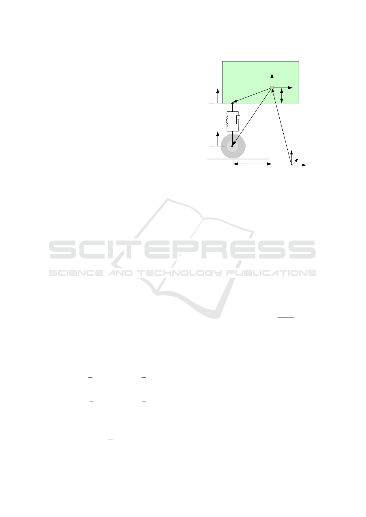
. The suspension of the right
rear wheel is shown in figure 3. The remaining sus-
pensions are modelled analogously. The related com-
ponents are
V
r
r
r
V B
f l
=
l
f
s
f
2
−s
z
,
V
r
r
r
V B
f r
=
l
f
−
s
f
2
−s
z
,
V
r
r
r
V B
rl
=
−l
r
s
r
2
−s
z
,
V
r
r
r
V B
rr
=
−l
r
−
s
r
2
−s
z
. (28)
The spring force is composed of a force law f (l
F
) and
the associated force direction e
e
e
F
F
F
F
F
= f (l
F
) ·
l
l
l
F
l
F
= f (l
F
) · e
e
e
F
. (29)
z
V
C
rr
D
rr
l
r
V
r
VB
rr
V
r
VW
rr
V
z
B
rr
z
W
rr
x
V
s
z
W
rr
B
rr
r
IVV
x
z
y
Figure 3: Suspension of the right rear wheel.
The direction of force is assumed to be perpendicular
to the road surface. For this reason, only the vertical
component of the vector z
B
j
=
I
r
r
r
IB
j
(3) is used in the
calculation of the spring force. The current length of
the suspension spring results from the vertical motion
of the attachment point on the vehicle body z
B
j
, the
position of wheel center point z
W
j
and the static spring
length l
stat
j
l
F
j
= z
B
j
− z
W
j
+ l
stat
j
. (30)
For example, the spring force of the left front wheel
with the relaxed spring length l
0
f l
yields to
V
F
F
F
F
f l
= −A
A
A
V I
·C
f l
·
0
0
z
B
f l
− z
W
f l
+ l
stat
f l
− l
0
f l
= A
A
A
V I
·
0
0
−C
f l
·
z
B
f l
− z
W
f l
+
l
r
·m
V
·g
2·l
(31)
The velocity of the attachment point of the suspen-
sion at the vehicle body is composed of the velocity
of the vehicle body and a component resulting from
its angular velocity
I
v
v
v
IB
j
=
I
v
v
v
IV
+
I
˜
ω
ω
ω
IV
·
I
r
r
r
V B
j
. (32)
In analogy to the spring force, only the vertical com-
ponent is considered in the calculation of the damper
force. This results with ˙z
B
j
=
I
v
v
v
IB
j
(3) in
V
F
F
F
D
j
= −A
A
A
V I
· D
j
·
0
0
˙z
B
j
− ˙z
W
j
. (33)
Due to the different deflection of the left and right
wheel of an axle, a force is induced in the roll stabi-
lizer, which tries to compensate this difference. For
SIMULTECH 2018 - 8th International Conference on Simulation and Modeling Methodologies, Technologies and Applications
406

the front and rear axle this leads to
V
F
F
F
S
f l
= −
V
F
F
F
S
f r
= −A
A
A
V I
·C
S
f
·
0
0
l
F
f l
− l
F
f r
; (34)
V
F
F
F
S
rl
= −
V
F
F
F
S
rr
= −A
A
A
V I
·C
S
r
·
0
0
l
F
rl
− l
F
rr
. (35)
The calculation of the tire slip resulting from the
tire-road contact requires the current position and the
speed of the wheel center. These kinematic variables
are described in the reference frame of the vehicle
body.
V
r
r
r
VW
j
=
V
r
r
r
V B
j
− A
A
A
V I
·
0
0
l
F
j
(36)
V
v
v
v
IW
j
=
V
v
v
v
IV
+
V
˜
ω
ω
ω
IV
·
V
r
r
r
VW
j
− A
A
A
V I
·
0
0
˙z
B
j
− ˙z
W
j
The computation of the tire slip, however, takes place
in the wheel-fixed reference frame, such that
W
v
v
v
IW
j
= A
A
A
WV
j
·
V
v
v
v
IW
j
(37)
is needed.
5 POWERTRAIN
To determine the temporal change of the angular ve-
locity of the driven wheels, the components of the
powertrain are needed. As an input only the desired
position of the accelerator pedal is to be specified,
which corresponds to the position of the throttle valve.
The behavior of the engine is described by the full
load characteristic and the speed-dependent curve of
the drag torque, which represents the friction losses in
the engine. The actual usable range is limited by the
idle speed. No torque can be transmitted below this
limit. The full load characteristic indicates the torque
that is available at the maximum accelerator pedal po-
sition (α
A
= 1). In most driving situations, however, a
lower torque is provided which can be approximated
using a nonlinear relationship
M
E
= M
Drag
· (1 − α
n
A
) + M
Full Load
· α
n
A
. (38)
The exponent n defines the characteristic of the curve.
The different shape types are listed in table 1. Taking
into account the mass moment of inertia of the engine
Θ
E
, the torque transmitted to the input shaft of the
clutch yields to
M
C
= M
E
− Θ
E
·
˙
ω
E
. (39)
Table 1: Shape of the engine torque curve.
• n = 1 → linear
• n < 1 → root shaped
• n > 1 → parabolic
The clutch consists of two discs (cf. figure 4). The
input clutch disk with the moment of inertia Θ
Cin
is
connected to the crankshaft and thus rotates with the
angular velocity of the engine ω
E
. The output clutch
shaft, which has a moment of inertia Θ
Cout
, may show
a different angular velocity ω
C
during the shifting
process. Since the shifting times are regarded as short
compared to the entire simulation time, it is assumed
that both clutch discs always have the same velocity.
The torque transmitted by the clutch is directly pro-
portional to the position of the clutch pedal α
C
. A
fully actuated clutch (α
C
= 1) ensures that the engine
is decoupled from the rest of the drive and no more
engine torque is transmitted. If the clutch is not actu-
ated, the entire engine torque acts on the output clutch
disc. The torque transmitted to the gearbox results in
M
G
=
M
C
−Θ
Cin
·
˙
ω
E
·(1 − α
C
)−Θ
Cout
·
˙
ω
C
. (40)
The gearbox consists of a manual transmission, a
transfer case and an axle drive. The rotating masses
of the gearbox are combined in two mass moments
of inertia. The transmission input shaft, together with
the gears mounted thereon, has the rotational inertia
Θ
Gin
. Due to the gear ratio i
G
, the transmission out-
put shaft with the mass moment of inertia Θ
Gout
has a
different angular velocity ω
G
ω
C
= i
G
· ω
G
. (41)
The torque transmitted from the gearbox to the trans-
fer case is given by
M
D
=
M
G
− Θ
Gin
·
˙
ω
C
· i
G
− Θ
Gout
·
˙
ω
G
. (42)
The transfer case distributes the generated torque to
the axles to be driven. The difference between the
several drive configurations is defined by a parameter
α
V
. If the vehicle has a front-wheel drive, the value is
zero. A rear-wheel drive uses α
V
= 1. The all-wheel
drive has a value in between. The axle drive with the
ratio i
D
is the last component of the powertrain. It
ensures that the same torque M
A
is transmitted to the
inner and outer wheels when cornering. The angular
velocity of the driven wheels can be determined from
ω
G
= i
D
· ω
D
=
i
D
2
· (ω
l
+ ω
r
). (43)
The corresponding torque results in
M
A
=
M
D
− Θ
Din
·
˙
ω
G
· i
D
− Θ
Dout
·
˙
ω
D
2
. (44)
Modeling and Validation of a Complex Vehicle Dynamics Model for Real-time Applications
407

M
E
α
A
Θ
E
Θ
Gin
ω
E
Θ
C
Θ
Cout
Θ
Cin
ω
G
Θ
Gout
i
G
i
D
Θ
W
Θ
W
ω
l
M
A
ω
r
M
A
Figure 4: Powertrain.
The driving torque acting on a front wheel is
M
A
k
= (1 − α
V
) · M
A
k = f l, f r. (45)
The torque that drives a rear wheel is given by
M
A
m
= α
V
· M
A
m = rl, rr. (46)
After the single components have been described,
they are assembled into an overall system. For this the
equations (39), (40), (42) and (44) are needed. With
(41) and (43) the angular velocity can be converted.
The total torque can be divided into two components
M
tot
= 2 ·M
A
= M
PT
− Θ
tot
·
˙
ω
D
. (47)
The first component represents the torque provided by
the engine
M
PT
= M
E
· (1 − α
C
) · i
G
· i
D
(48)
and the second component considers the total mass
moment of inertia of the powertrain, which counter-
acts a change of the angular velocity
Θ
tot
=
(Θ
E
+ Θ
Cin
) · (1 − α
C
) + Θ
Cout
+Θ
Gin
· i
2
G
+ Θ
Gout
+ Θ
Din
· i
2
D
+ Θ
Dout
. (49)
The mass moment of inertia reduced to a wheel of
the front axle consists of the rotational inertia of the
front wheel θ
W
f
and a component resulting from the
powertrain
Θ
totW
k
= Θ
W
f
+
1 − α
V
2
· Θ
tot
k = f l, f r. (50)
The total rotational mass moment of inertia of a rear
wheel results in
Θ
totW
m
= Θ
W
r
+
α
V
2
· Θ
tot
m = rl, rr. (51)
6 TIRE BEHAVIOR
6.1 Wheel Load
The wheel load F
z
j
consists of two components. The
static component results from the mass distribution of
the vehicle body m
V
and the weight of a wheel and
its associated wheel carrier, which are summarized in
m
W
j
· g. The dynamic component considers the loads
that arise in the suspensions as a result of the pitch
and roll of the vehicle body:
F
z
f l
=
m
V
· l
r
2 · l
+ m
W
f
· g −C
f l
· z
f l
− D
f l
· ˙z
f l
F
z
f r
=
m
V
· l
r
2 · l
+ m
W
f
· g −C
f r
· z
f r
− D
f r
· ˙z
f r
F
z
rl
=
m
V
· l
f
2 · l
+ m
W
r
· g −C
rl
· z
rl
− D
rl
· ˙z
rl
F
z
rr
=
m
V
· l
f
2 · l
+ m
W
r
· g −C
rr
· z
rr
− D
rr
· ˙z
rr
(52)
The parameter l
f
and l
r
denote the distance between
the center of gravity of the vehicle body and the front
and rear axle. The wheelbase is characterized by l.
The spring deflection results from the relative motion
between the attachment point of the wheel suspension
at the vehicle body z
B
j
and the tire deflection z
W
j
.
z
j
= z
B
j
− z
W
j
(53)
˙z
j
= ˙z
B
j
− ˙z
W
j
(54)
SIMULTECH 2018 - 8th International Conference on Simulation and Modeling Methodologies, Technologies and Applications
408
6.2 Horizontal Wheel Force
For the transmission of the horizontal forces in the
contact area between the tire and the road, friction is
necessary. The most important physical effects that
are responsible for those forces are adhesion and hys-
teresis friction (Gillespie, 1992). The first component
is based on intermolecular bonding between the rub-
ber of the tire and the road surface. The second part
results in a form fit due to meshing of the tire contact
patch and the road surface. Pure longitudinal forces
F
W x
j
only appear when driving straight ahead. Pure
lateral forces F
Wy
j
occur for freely rolling wheels. In
all other driving situations, there is a superposition of
the two forces. The maximum transmissible horizon-
tal forces in the tire longitudinal and lateral direction
are assumed to be proportional to the friction coeffi-
cient µ
max
j
F
H
j
=
q
F
2
W x
j
+ F
2
Wy
j
= µ
max
j
· F
z
j
. (55)
6.3 Slip Computation
A measure of the amount of sliding motion that occurs
between the tire and the road are the longitudinal slip
κ
j
and the lateral slip α
j
. The relative motion in lon-
gitudinal direction is based on the difference in speed
between the rolling motion of the wheel with the dy-
namic tire radius r
dyn
j
and the translational velocity
of the wheel center v
W x
j
v
di f f
j
= v
W x
j
−
˙
ρ
W
j
· r
dyn
j
. (56)
In most driving maneuvers, the driver performs a ve-
hicle intervention that abruptly changes the current
driving state. This results in a deformation of the tire
in the longitudinal direction u and in the lateral direc-
tion w. A stationary state only sets in with time delay.
This behavior is approximated by a first-order lag be-
havior. The resulting equations are
σ
κ
j
·
du
j
dt
+ |v
W x
j
| · u
j
= −σ
κ
j
· v
di f f
j
(57)
σ
α
j
·
dw
j
dt
+ |v
W x
j
| · w
j
= σ
α
j
· v
Wy
j
. (58)
The relaxation lengths σ
κ
j
and σ
α
j
can be determined
using the parameters of the tire model Magic Formula
(Pacejka and Besselink, 2012). The longitudinal slip
κ
j
and the lateral slip α
j
can be specified from the
solution of the differential equations (57) and (58).
κ
j
=
u
j
σ
κ
j
· sgn(v
di f f
j
) (59)
α
j
= atan
w
j
σ
α
j
!
(60)
6.4 Tire Model Magic Formula
After the kinematics of the tire-road contact is known
by the two slip variables, the effective forces and
torques in the contact area should now be calculated.
Therefore, a model of the tire behavior is needed.
On the one hand there are physical tire models like
(Gipser, 2007) and (Baecker et al., 2010), which take
into account the processes in the tire and therefore
require a long computing time. On the other hand,
there are empirical models like (Hirschberg et al.,
2007) and (Pacejka and Besselink, 2012). These at-
tempt to describe the characteristics measured on a
tire test bench using mathematical approaches that
are preferably composed of algebraic or trigonomet-
ric functions without taking the physical properties
of the tire into account. This ensures that signifi-
cantly less computation time is needed and a real-
time computation is much easier to realize. Conse-
quently, the empirical tire model Magic Formula is
used here. It is widespread and offers a variety of key
figures and influencing factors that allow a good ap-
proximation to the real tire behavior. In the following,
only a rough overview is given and the basic structure
is presented. Further information and all the equa-
tions needed for the computation of the individual pa-
rameters described here can be found in (Pacejka and
Besselink, 2012).
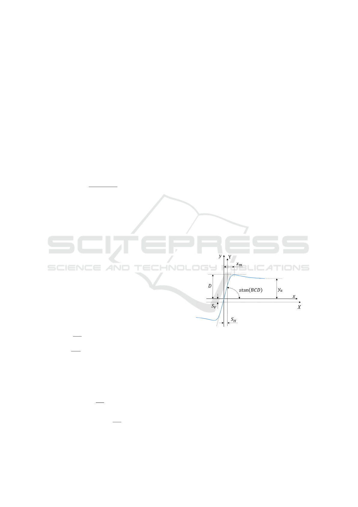
Figure 5: Tire behavior.
The Magic Formula model uses a mathematical ap-
proach to describe the tire forces and torques based on
the trigonometric functions sine and arctangent. A re-
alistic approximation of a measured curve is achieved
by a suitable choice of the parameters B, C, D, E.
These values take into account various influencing
factors such as a variation of the wheel load F
z
, cam-
ber γ, longitudinal slip κ and lateral slip α. The basic
equation of the Magic Formula is
y = D · sin
C · arctan
B · x − E ·
B · x
− arctan(B · x)
.
(61)
Modeling and Validation of a Complex Vehicle Dynamics Model for Real-time Applications
409
The characteristic curve in figure 5 may be shifted
around the origin due to asymmetries in the tire struc-
ture
X = x + S
H
Y = y + S
V
. (62)
The parameter D represents the maximum value of
the tire characteristics. It depends on the wheel load
and the friction coefficient. The product of the three
parameters B · C · D correlates with the slope of the
curve at the origin. The shape factor C is calculated
from the height of the asymptote y
a
and influences the
limit of the range of the sine function
C = 1 ±
1 −
2
π
· arcsin
y
a
D
. (63)
The parameter B determines the slope at the origin
and therefore it is called stiffness factor. The value of
E specifies the curvature at the maximum of the curve
E =
B · x
m
− tan
π
2·C
B · x
m
− arctan(B · x
m
)
. (64)
The longitudinal and lateral forces are not indepen-
dent of each other, since the lateral slip has an in-
fluence on the longitudinal force and the longitudinal
slip on the lateral force. This fact is taken into account
by the weighting factors G
xα
and G
yκ
. This leads to
the tire longitudinal force
F
W x
= G
xα
· F
W x0
+ S
vxα
. (65)
The weighting factor G
xα
is chosen to be one if there
is no lateral slip
G
xα
=
cos
C
xα
· arctan
B
xα
· (α + S
Hx α
)
cos
C
xα
· arctan
B
xα
· S
Hx α
. (66)
F
W x0
represents the tire force, which appear for pure
longitudinal slip. S
vxα
describes the offset force. The
same applies to the side force. This results in
F
Wy
= G
yκ
· F
Wy0
+ S
vyκ
; (67)
G
yκ
=
cos
C
yκ
· arctan
B
yκ
· (κ + S
Hyκ
)
cos
C
yκ
· arctan
B
yκ
· S
Hyκ
. (68)
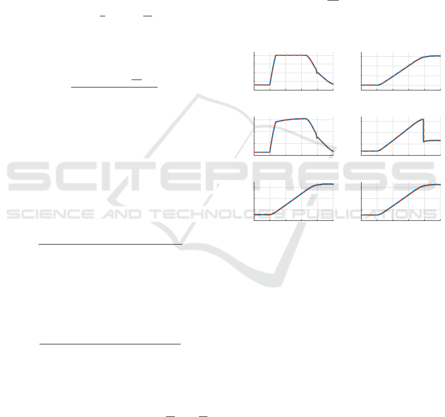
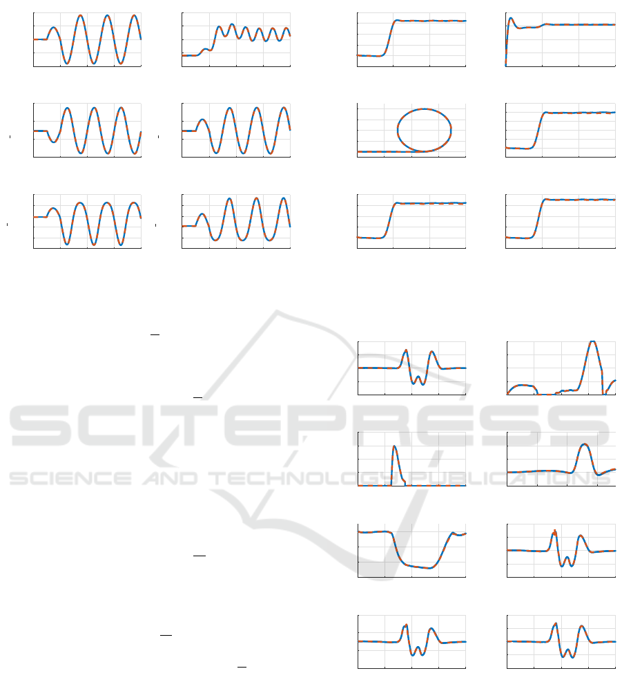
7 VALIDATION
In figure 6 the vehicle accelerates from 50
km
h
to 80
km
h
.
The presented parameters show a high correlation be-
tween the Matlab and the CarMaker model. The cur-
rent position of the accelerator pedal, which is re-
quired as an input signal of the powertrain model, is
extracted from CarMaker. At the beginning, the ac-
celerator pedal position is constant for two seconds.
Thereafter, the value is increased to the maximum
value 1 over a period of 0.8 seconds. The signal is
then constant for about 4 seconds. After the gear
change, it decreases again. The engine torque has
a similar curve progression. Due to the exponent of
0.80, the calculation of the currently available torque
in (38) results in a degressive course. The maximum
relative error in the engine torque between the both
models is about 3% and occurs when the driver starts
accelerating. A reason for this is the dead time in the
CarMaker System which is neglected in Matlab. If
a engine speed of 3800
1
min
is reached, a gear change
takes place. As a result, the velocity drops abruptly.
The angular velocity shows a similar behavior as the
longitudinal velocity.
0 2 4 6 8 10
t [s]
0
0.25
0.5
0.75
1
α
A
[−]
Accelerator position
0 2 4 6 8 10
t [s]
50
60
70
80
v
x
[km/h]
Longitudinal velocity
0 2 4 6 8 10
t [s]
0
40
80
120
M
E
[Nm]
Engine torque
0 2 4 6 8 10
t [s]
2200
2700
3200
3700
n
E
[1/min]
Engine speed
0 2 4 6 8 10
t [s]
40
50
60
70
ω
fl
[rad/s]
Angular velocity front left
0 2 4 6 8 10
t [s]
40
50
60
70
ω
fr
[rad/s]
Angular velocity rear left
Figure 6: Validation of the powertrain model during an ac-
celeration process: CarMaker (red); Matlab (blue).
The process of sinusoidal steering (cf. figure 7) starts
after driving straight ahead for two seconds. The ac-
tual driving maneuver takes 14 seconds. The am-
plitude of the first half sine is half of the following
three oscillation periods. If the steering angle were
the same as the first one, the vehicle would drift off
to one side because the direction of the vehicle would
not be reversed. The curve progression of the wheel
loads of the left and right front wheels behave sym-
metrically to the value that occurs in a pure longitudi-
nal motion. The maximum relative error of the wheel
load is about 1.5% und the absolute error is 45 N.
In order to obtain a stationary driving behavior, which
is a prerequisite for a steady-state circular test, the ve-
hicle in figure 8 drives straight ahead for 250 m. Then
a circular path with a radius of 100 m is followed.
Within ten seconds there is a smooth transition be-
tween the straight section and the circle. In this tran-
sitional period, the lateral acceleration increases and
SIMULTECH 2018 - 8th International Conference on Simulation and Modeling Methodologies, Technologies and Applications
410
0 4 8 12 16
t [s]
-100
-50
0
50
100
δ
SW
[
◦
]
Steering wheel angle
0 4 8 12 16
t [s]
0.12
0.15
0.18
0.21
0.24
α
A
[−]
Accelerator position
0 4 8 12 16
t [s]
2000
3000
4000
5000
F
z f l
[N]
Wheel load front left
0 4 8 12 16
t [s]
2000
3000
4000
5000
F
z f r
[N]
Wheel load front right
0 4 8 12 16
t [s]
-3000
-2000
-1000
0
1000
2000
F
W y f l
[N]
Lateral force front left
0 4 8 12 16
t [s]
-2000
-1000
0
1000
2000
3000
F
W y f r
[N]
Lateral force front right
Figure 7: Validation of the tire forces during a sinusoidal
steering: CarMaker (red); Matlab (blue).
finally reaches a value of 2
m
s
2
in the CarMaker model,
which remains the same over the entire period. In the
Matlab model, the lateral acceleration is slightly in-
creasing. The maximum occurring relative error is
3% and the absolute error is 0.06
m
s
2
. The roll angle
shows a similar behavior (relative error 2.8% and ab-
solute error 4 · 10
−4
rad). The yaw rate is almost the
same in both models. Despite the deviations between
the two models, there is no significant difference in
the trajectory of the vehicle. This indicates a stable
behavior of the Matlab model for the use in longer
simulations.
Furthermore, the vehicle behavior is analyzed in an
evasive maneuver (cf. 9). At the beginning, the ve-
hicle is moving at a speed of 50
km
h
straight ahead.
However, this is too fast to drive through the course.
For this reason, a braking process is necessary. Af-
ter the obstacle is avoided, the vehicle is acceler-
ated again. The maximum absolute error occurring in
the speed progression is 0.5
km
h
and the relative error
1.3%. The lateral acceleration shows only a visible
deviation at 8.8 seconds (absolute error 0.1
m
s
2
, relative
error 4.0%). The difference is due to the fact that in
the Matlab model the duration for the gear change is
neglected. The roll angle and the yaw rate, however,
show no difference.
Although the vehicle model has been validated only
by comparison with a program system such as Car-
Maker, there are no limitations for the use in real-
world simulations. The external influences like the
wind are represented by the aerodynamics. The to-
pography of the road is taken into account by the
climbing resistance. The biggest uncertainties of the
vehicle model are the parameters that occur in the
0 20 40 60
t [s]
-10
0
10
20
30
40
δ
SW
[
◦
]
Steering wheel angle
0 20 40 60
t [s]
0
0.05
0.1
0.15
0.2
α
A
[-]
Accelerator position
0 100 200 300 400
x [m]
0
50
100
150
200
y [m]
Horizontal motion
0 20 40 60
t [s]
-0.5
0
0.5
1
1.5
2
2.5
a
y
[m/s
2
]
Lateral acceleration
0 20 40 60
t [s]
-4
0
4
8
12
16
φ [rad]
×10
−3
Roll angle
0 20 40 60
t [s]
-0.04
0
0.04
0.08
0.12
0.16
˙
ψ [rad/s]
Yaw rate
Figure 8: Validation of the vehicle parameter during a cir-
cular test: CarMaker (red); Matlab (blue).
0 5 10 15 20
t [s]
-200
-100
0
100
200
δ
SW
[
◦
]
Steering wheel angle
0 5 10 15 20
t [s]
0
0.25
0.5
0.75
1
α
A
[-]
Accelerator position
0 5 10 15 20
t [s]
0
0.1
0.2
0.3
0.4
α
B
[-]
Brake pedal position
0 50 100 150
x [m]
-2
0
2
4
6
y [m]
Horizontal motion
0 5 10 15 20
t [s]
20
30
40
50
v
x
[km/h]
Longitudinal velocity
0 5 10 15 20
t [s]
-4
-2
0
2
4
a
y
[m/s
2
]
Lateral acceleration
0 5 10 15 20
t [s]
-0.03
-0.01
0.01
0.03
φ [rad]
Roll angle
0 5 10 15 20
t [s]
-0.5
-0.25
0
0.25
0.5
˙
ψ [rad/s]
Yaw rate
Figure 9: Validation of the vehicle parameter during an eva-
sive maneuver: CarMaker (red); Matlab (blue).
single vehicle components. These have be deter-
mined experimentally on a test track before the ve-
hicle model is used in real-world simulations.
Modeling and Validation of a Complex Vehicle Dynamics Model for Real-time Applications
411
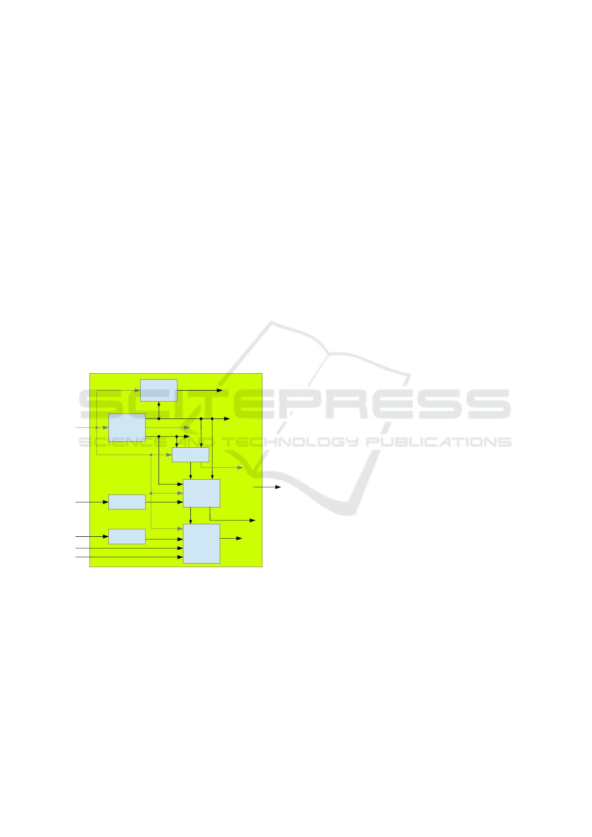
8 PROGRAM STRUCTURE AND
REAL-TIME CAPABILITY
When determining the structure of the source code,
great emphasis was put on both computing speed and
usability. The strucure of the vehicle model imple-
mented in Matlab is shown in figure 10. In the main
file, only the temporal change of the state vector is
determined, which is described by the kinematic and
dynamic equations of motion. Furthermore, the kine-
matics and dynamics in vector-matrix form are used
to reduce the number of equations. The occurring pa-
rameters are determined in subroutines. The compo-
nents described in the previous chapters, such as the
powertrain or the tire model, are stored in separate
files, so that they can easily be replaced if the vehicle
configuration changes. Values such as the wheel load,
which are required both for the calculation of the tire
forces in the longitudinal and lateral direction and for
the vertical motion of the wheel, are located in one of
the upper program levels. Thereby, all program parts
that need this information can access it and a recal-
culation is avoided. At the beginning the start values
Steering
Brake
Suspension
Wheel
Driving
Resistance
Kinematics
Powertrain
z
u
A
IV
ω
IVV
α
B
M
B
j
δ
SW
δ
M
DRV
F
DRV
F
dyn
j
W
F
FD
j
V
M
FD
j
V
M
Wy
j
F
VW
j
V
α
A
˙
ω
j
dz
F
Wx
j
M
VW
j
V
α
C
Figure 10: Structure of the Matlab model.
of the state vector z
z
z have to be defined. In addition,
the temporal courses of the accelerator pedal position,
the brake pedal position and the steering wheel angle
are to be specified as input data for the vehicle model.
At each time step, the change of the state vector d
d
dz
z
z
is determined. This first order differential equation is
then solved by means of the Matlab solver ode45 with
a time increment of one millisecond. The state vector
obtained thereby is the input for the next simulation
step.
One of the fundamental conditions to the nonlinear
twin track model presented in this paper is the real-
time capability. For this purpose, the computing time
required for the maneuvers for validating the vehicle
model is analyzed. To create the results listed in ta-
ble 2, the mean of five simulations is calculated us-
ing a laptop with the characteristics(Intel (R) Core
(TM) i5-7200U CPU)@ 2.50GHz 2.71GHz on a 64-
bit Windows operating system. The results show that
the vehicle dynamics model developed here enables
a real-time simulation for all driving maneuvers pre-
sented here. In order to achieve a further reduction in
Table 2: Real-time capability.
Maneuver Real Matlab mex
Acceleration [s] 10 2.72 0.46
Sinusoidal steering [s] 16 5.59 0.93
Circular test [s] 70 15.33 2.69
Evasive maneuver [s] 20 6.63 1.02
the computing time, the vehicle model is transferred
to the C programming language. The resulting file is
then integrated into Matlab as a mex file. The com-
puting speed is increased by a factor of 5.7.
9 CONCLUSION
In this paper, a nonlinear twin track model has been
introduced, containing all the components that are im-
portant for the vehicle handling. All components and
the entire vehicle has been compared to the CarMaker
system. The tire forces are validated by a sinusoidal
steering. The powertrain has used an acceleration pro-
cess for validation. All considered parameters show
no significant difference between the both systems.
The quality of the modeling of the behavior of the ve-
hicle body, which also takes into account the vertical
dynamics in addition to the horizontal dynamics, has
been evaluated by a driving maneuver, which consists
of a straight-ahead and a circular driving, and by an
evasive maneuver. In the first one, there are small de-
viations in the roll angle and in the lateral accelera-
tion, which are not constant during the circular driv-
ing and still increase slightly. In second maneuver one
there is no difference. The computation time fulfills
the requirement of a real-time simulation as a function
of the illustrated maneuvers. The remaining computa-
tion time may be used in future projects to implement
a controller that generates the required input variables
of the vehicle model based on a predetermined trajec-
tory and a speed profile. Furthermore, a method need
to be developed to determine the required parameters
of the nonlinear two-track model with reasonable ef-
fort on a proving ground.
SIMULTECH 2018 - 8th International Conference on Simulation and Modeling Methodologies, Technologies and Applications
412

ACKNOWLEDGEMENT
This work was supported by the German Federal Min-
istry of Education and Research.
REFERENCES
Baecker, M., Gallrein, A., and Haga, H. (2010). A tire
model for very large tire deformations and its applica-
tion in very severe events. SAE International Journal
of Materials and Manufacturing, 3(1):142–151.
Gillespie, T. D. (1992). Fundamentals of vehicle dynamics.
Society of Automotive Engineers, Warrendale, PA, 4.
printing edition.
Gipser, M. (2007). Ftire – the tire simulation model for
all applications related to vehicle dynamics. Vehicle
System Dynamics, 45(sup1):139–151.
Hirschberg, W., Rill, G., and Weinfurter, H. (2007).
Tire model tmeasy. Vehicle System Dynamics,
45(sup1):101–119.
Pacejka, H. B. and Besselink, I. (2012). Tire and vehicle
dynamics. Elsevier/BH, Amsterdam and Boston, 3rd
ed. edition.
Popp, K. and Schiehlen, W. (1993). Fahrzeugdy-
namik: Eine Einf
¨
uhrung in die Dynamik des Sys-
tems Fahrzeug - Fahrweg ; mit 27 Beispielen, vol-
ume 70 of Leitf
¨
aden der angewandten Mathematik
und Mechanik. Teubner, Stuttgart.
Schramm, D., Hiller, M., and Bardini, R. (2018). Vehicle
Dynamics: Modeling and Simulation. Springer, Ber-
lin, Heidelberg and s.l., 2nd ed. 2018 edition.
Modeling and Validation of a Complex Vehicle Dynamics Model for Real-time Applications
413
