
Supporting the Systematic Goal Refinement in KAOS using the
Six-Variable Model
Nelufar Ulfat-Bunyadi, Nazila Gol Mohammadi and Maritta Heisel
University of Duisburg-Essen, Duisburg, Germany
Keywords:
Domain Knowledge, Assumption, Domain Hypothesis, Context, Context Modelling.
Abstract:
In requirements engineering, different types of modelling techniques exist for documenting requirements and
their refinement (e.g. goal-oriented techniques, problem-based techniques). Each type of technique has its
advantages and shortcomings. However, extensions made to one type may be beneficial to another type as
well, if transferred to it. KAOS is, for example, a comprehensive methodology that supports goal-oriented
requirements engineering. As part of the KAOS methodology, multi-agent goals are refined until they can
be assigned to single agents in the software or in the environment. Beside goals, domain properties and
hypotheses (facts and assumptions about the environment) can also be modelled in KAOS goal models as well
as their influence on the satisfaction of goals. However, the KAOS methodology provides limited support in the
systematic refinement of goals. Developers using the KAOS method are left alone in refining the multi-agent
goals and in making domain properties and hypotheses explicit. The Six-Variable Model, on the other hand,
is an extension of problem diagrams and supports a systematic refinement of requirements and a systematic
elicitation of domain properties and domain hypotheses. In this paper, we show how the Six-Variable Model
can be used to support a systematic refinement of goals in KAOS goal models.
1 INTRODUCTION
KAOS is a goal-oriented requirements engineering
methodology that was developed by van Lamsweerde
(van Lamsweerde, 2009). Problem diagrams have
been introduced by Jackson (Jackson, 2001) as part of
the problem frames method. Both methods are inten-
ded to support early requirements engineering. KAOS
goal models and problem diagrams are both based
on the well-known satisfaction argument which was
originally developed by Zave and Jackson (Zave and
Jackson, 1997). This commonality facilitates combi-
ning them and transferring or using concepts like the
Six-Variable Model (Ulfat-Bunyadi et al., 2016), de-
fined for problem diagrams, for goal models as well
to overcome shortcomings like the lack of support for
a systematic refinement of goals.
As regards the refinement of goals in KAOS goal
models, van Lamsweerde (van Lamsweerde, 2009)
suggests some heuristics to support this task. One
heuristic consists in asking HOW questions (e.g. How
can a goal G be satisfied? Is this subgoal sufficient or
is there any other subgoal needed for satisfying G?).
Another heuristic which has similarities with the work
we present in this paper is called Split responsibili-
ties. According to this heuristic, a goal is refined into
subgoals by requiring the subgoals to involve fewer
potential agents in their satisfaction than the parent
goal. However, these are only heuristics. A syste-
matic approach for achieving such a refinement and
arriving at such subgoals is not provided. Our method
fills this gap.
The paper is structured as follows. In Section 2,
we first introduce the fundamentals of our work. In
Sections 3, we present our method and illustrate its
application using an example. In Section 4, we dis-
cuss related work. Finally, in Section 5, we provide a
conclusion and an outlook on future work.
2 BACKGROUND
In this section, we introduce the satisfaction argu-
ment, KAOS goal models, problem diagrams, and the
Six-Variable Model.
The Satisfaction Argument. Zave and Jackson
(Zave and Jackson, 1997) differentiate between the
system, the machine, and the environment. The ma-
chine is the software-to-be. The environment is a
part of the real world whose current behaviour is
102
Ulfat-Bunyadi, N., Mohammadi, N. and Heisel, M.
Supporting the Systematic Goal Refinement in KAOS using the Six-Variable Model.
DOI: 10.5220/0006850701020111
In Proceedings of the 13th International Conference on Software Technologies (ICSOFT 2018), pages 102-111
ISBN: 978-989-758-320-9
Copyright © 2018 by SCITEPRESS – Science and Technology Publications, Lda. All rights reserved

unsatisfactory. The software-to-be will be integrated
into this environment to solve this problem. Then,
the behaviour of the environment will be satisfactory.
The software-to-be and its environment, together, re-
present the system. There are three types of state-
ments about the system, the software-to-be, and the
environment: the specification S, the domain know-
ledge D, and the requirements R. Based on these sta-
tements, the satisfaction argument is defined as fol-
lows: S, D ` R. The argument says that, if a software
is developed which satisfies S and is integrated into
an environment as described by D, and S and D are
consistent with each other, then R is satisfied.
KAOS Goal Models. Van Lamsweerde (van Lam-
sweerde, 2009) calls S software requirements and R
system requirements. As regards domain knowledge,
he distinguishes between: domain properties, dom-
ain hypotheses, and expectations. Domain properties
are facts about the environment (e.g. physical laws),
while domain hypotheses and expectations are both
assumptions about the environment. A domain hypot-
hesis is a descriptive statement about the environment
which simply needs to hold. An expectation is a pres-
criptive statement about the environment and, in con-
trast to domain hypotheses which are to be satisfied
by the environment in general, can be assigned to a
concrete agent in the environment who is responsible
for satisfying it (e.g. to a sensor, actuator, the user).
A KAOS goal model is an AND/OR graph. An
example is shown in Figure 9. Nodes of the graph are
multi-agent goals (i.e. goals that are further refined),
single-agent goals (i.e. leaf goals which are either as-
signed to the software-to-be (then they are software
requirements) or to the environment (then they are ex-
pectations)), domain properties, or domain hypothe-
ses. The AND/OR-refinement relationships between
the nodes show which subgoals need to be satisfied
and which domain properties and domain hypotheses
need to be valid to satisfy a parent goal. Thus, the
goal refinement structure reflects Zave and Jackson’s
satisfaction argument.
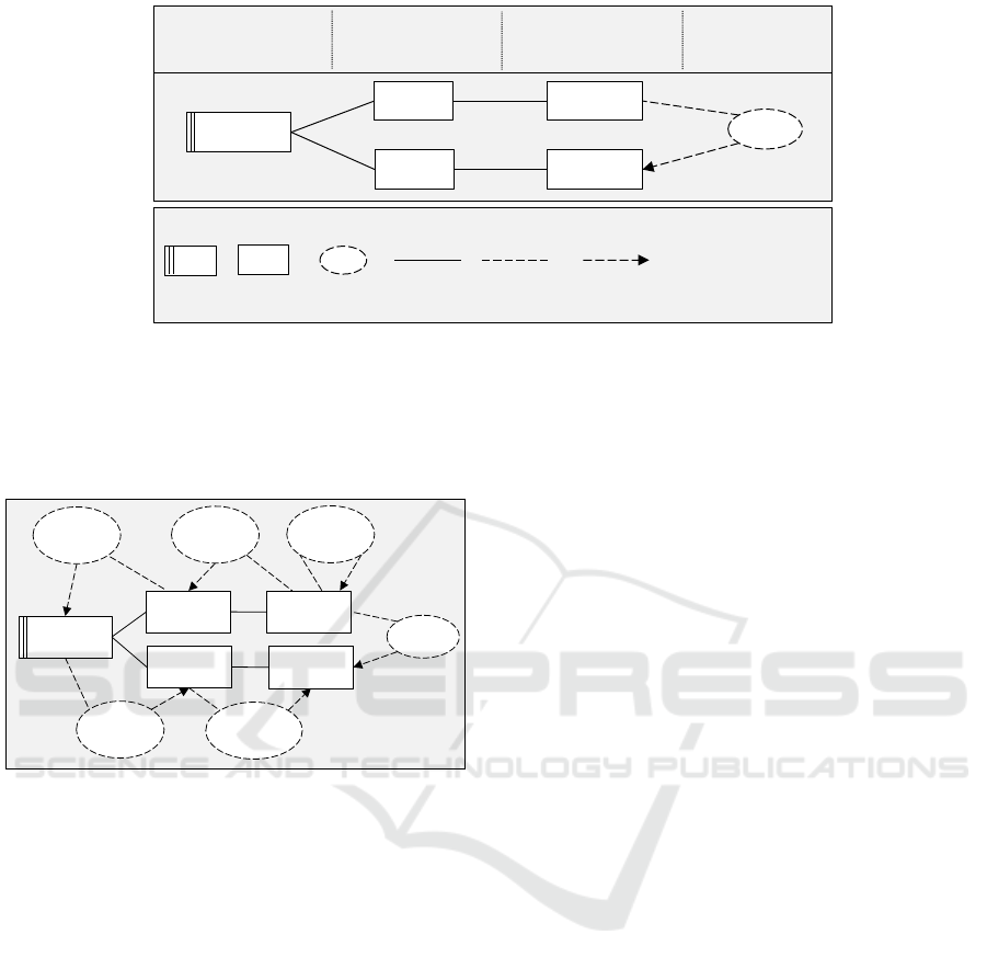
Problem Diagrams. Problem diagrams have been
suggested by Jackson (Jackson, 2001). They show the
software-to-be, the requirement to be satisfied in the
environment, and the part of the environment which
is relevant for satisfying the requirement. The nota-
tion is shown in Figure 1 and an example of a pro-
blem diagram is shown in Figure 6. The software-
to-be is shown as a so-called machine domain, the
environment is shown in terms of so-called problem
domains (material and immaterial objects in the en-
vironment) which are directly or indirectly connected
to the machine domain, and the requirement is shown
as a dashed oval connected to some problem dom-
ains. Three types of connections are differentiated:
interfaces, requirement references, and constraining
references. Interfaces exist between problem and ma-
chine domains where phenomena (events, states, va-
lues) are shared. Sharing means that one domain ob-
serves the phenomena, while the other controls them.
The controlling domain is annotated at the interface
(using an abbreviation followed by an exclamation
mark) as well as the phenomena. Requirement refe-
rences and constraining references, each connect the
requirement with problem domains. A requirement
reference is used to express that the requirement refers
to phenomena of the problem domain. A constraining
reference is used to express that the requirement con-
strains phenomena of the problem domain.
The Six-Variable Model. The Six-Variable Mo-
del (Ulfat-Bunyadi et al., 2016) is based on the
well-known Four-Variable Model (Parnas and Madey,
1995) and focuses on control systems. A control sy-
stem consists of some control software which uses
sensors and actuators to monitor/control certain quan-
tities in the environment. The Four-Variable Model
differentiates between four variables: monitored va-
riables m (environmental quantities the control soft-
ware monitors through input devices), controlled va-
riables c (environmental quantities the control soft-
ware controls through output devices), input variables
i (data items that the control software needs as input),
and output variables o (quantities that the control soft-
ware produces as output).
Frequently, it is not possible to monitor/control
exactly those variables one is interested in. Instead,
a different set of variables is monitored/controlled,
whose variables are related to the ones of real inte-
rest. The Six-Variable Model demands that the vari-
ables of real interest should be documented as well
(beside the classical four variables). The two addi-
tional variables are r and d. r (referenced) variables
are environmental quantities that should originally be
observed in the environment. Originally means before
deciding which sensors/actuators/other systems to use
for monitoring/controlling. d (desired) variables are
environmental quantities that should originally be in-
fluenced in the environment. The Six-Variable Model
is depicted in Figure 1 as a problem diagram.
For problem diagrams created based on the Six-
Variable model, the domain hypotheses, expectations,
and software requirements can be made explicit as
shown in Figure 2. DH-MD is a hypothesis about the
monitored domain, which needs to be true. Exp-SE
is an expectation to be satisfied by the sensors, Exp-
AC is an expectation to be satisfied by the actuators,
and Exp-CD is an expectation to be satisfied by the
controlled domain. SOF represents the software re-
Supporting the Systematic Goal Refinement in KAOS using the Six-Variable Model
103
Control
machine
Monitored
domain
REQ
Controlled
domain
SE!{i}
CM!{o}
Sensor
MD!{m}
MD!{r}
Actuator
CD!{d}
AC!{c}
Used sensors/
actuators/
other systems
Requirement
in environment
Software-to-be
Problem
domains
in environment
Legend:
Machine
domain
Problem
domain
InterfaceRequirement Requirement
reference
Constraining
reference
r: referenced variables
d: desired variables
m: monitored variables
c: controlled variables
i: input variables
o: output variables
Figure 1: The Six-Variable Model (Ulfat-Bunyadi et al., 2016).
quirements which are to be satisfied by the control
machine. The requirements REQ can only be satis-
fied, if DH-MD is valid and Exp-SE, SOF, Exp-AC as
well as Exp-CD are satisfied.
DH-MD: m
actually
reflects r
r
m
Control
machine
Monitored
domain
REQ
i
o
Sensor
m
r
Actuator
c
Controlled
domain
d
Exp-SE: i
actually
corresponds
to m
i
m
Exp-AC: o
actually
results in c
o
c
Exp-CD: d is
actually
achieved by c
c
d
SOF:
produce o
from i
o
i
Satisfaction argument: DH-MD, Exp-SE, SOF, Exp-AC, Exp-CD ├ REQ
Figure 2: Assumptions in the Six-Variable Model (Ulfat-
Bunyadi et al., 2016).
3 METHOD AND APPLICATION
In this section, we first elaborate on the benefit of
combining goal models and problem diagrams in ge-
neral. Then, we show how KAOS goal models and
problem diagrams can actually be combined in a sys-
tematic way, i.e. we present our method and its appli-
cation to an example. Finally, we describe the benefit
of our method.
3.1 Our Method
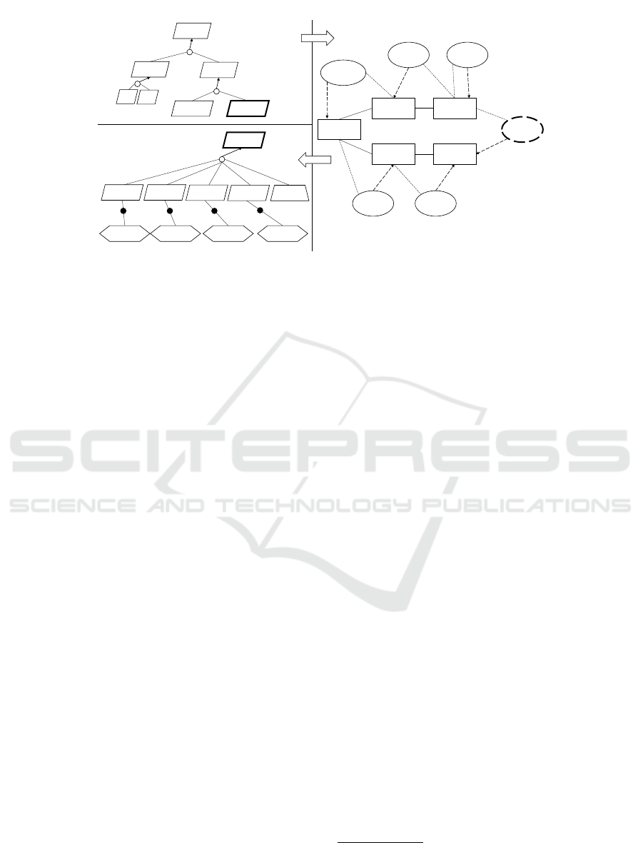
As mentioned above, KAOS goal models and problem
diagrams have in common that they are both based on
the satisfaction argument. We exploit this commo-
nality for refining goals in KAOS goal models in a
systematic way (see Figure 3).
Since goals typically represent stakeholder inten-
tions, they are very helpful in initially eliciting the
effects that shall be achieved in the real world, the
environment. The system is developed to solve a pro-
blem in the environment. Therefore, the effects that
shall be achieved there need to be elicited as a first
step during software development. Another advan-
tage of goal models is that they make explicit how
goals depend on each other, i.e. which goals con-
tribute to the satisfaction of other goals. If the goal
model captures not only goals but also requirements,
expectations, domain properties, and domain hypot-
heses as it is the case in KAOS goal models, then the
dependencies among these is visible as well, i.e. it
is clear which domain properties and hypotheses as
well as requirements and expectations need to be va-
lid/satisfied to satisfy the parent goal.
The benefit of problem diagrams which are cre-
ated based on the Six-Variable Model is that the six
variables are made explicit therein. This information
is missing in KAOS goal models. Based on the six
variables, the expectations, domain hypotheses, and
domain properties can be made explicit more easily
because they are actually statements describing the
relation between two or more variables. For exam-
ple, the relation between r and m is usually a domain
hypothesis, if r and m are different (e.g. if a variable
m is monitored which is only an estimation of r).
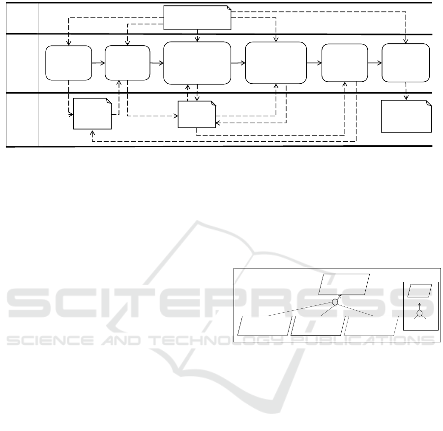
An overview of our method for the systematic re-
finement of goals is shown in Figure 4. It consists
of six steps that we describe in the following in more
detail.
Step 1: Create Initial KAOS Goal Model. As a first
step, an initial KAOS goal model is created. This ini-
tial goal model focuses solely on the effects that shall
be achieved in the real world. This means that, during
this step, it is not important how these effects might
be achieved, i.e. by means of which technology. So-
lutions like sensors, actuators, or other systems to be
used are not considered.
Step 2: Make Six Variables Explicit. During this step,
ICSOFT 2018 - 13th International Conference on Software Technologies
104
G2
G2.1 G2.2
SofReq Exp-SE
DH
Machine
G2.2
Env. Mon.Sensor
Env. Con.Actuator
Machine
DH
Exp-
SE
Exp-
AC
Exp-
EC.
SofReq
Exp-AC
Exp-EC
Sensor Actuator
Env. Con.
G0
G1
…
…
KAOS Goal Model
Problem Diagram based on Six-Variable Model
G2.2
Figure 3: Combination of KAOS goal models and problem diagrams.
solutions for achieving the leaf goals shown in the
initial goal model from Step 1 are considered. For
each leaf goal, a problem diagram is created based on
the Six-Variable Model. Note that the number of va-
riables depends on the number of problem domains
that exist between the machine domain, on the one
hand, and the so-called real world domains, on the
other hand. By real world domain, we mean a pro-
blem domain in the environment of the machine that
is either the source of stimuli for the machine or the
sink of responses created by the machine. In contrast
to that, sensors and actuators are, for example, usually
not real world domains, because these are only means
for observing phenomena of real world domains or
achieving effects on real world domains. Thus, they
are not the sources/sinks but rather problem domains
connecting the machine domain to real world dom-
ains. Note that there might, for example, be chains
of sensors or actuators and thus, there might not only
be six variables (i.e. the classical 4 plus 2 additional
ones), but 4 + n variables to be documented.
Step 3: Decompose Problem Diagram based on Refe-
renced and Desired Phenomena. Sometimes the pro-
blem diagrams resulting from Step 2 are still too com-
plex to make expectations, domain hypotheses, and
software requirements explicit (Step 4). This mani-
fests itself in complex expectations, domain hypot-
heses, and especially in complex software require-
ments. This is always a hint for further decomposing
the requirement. The decomposition has the advan-
tage that important expectations, domain hypotheses,
and software requirements are not forgotten or over-
looked due to complexity of the requirement (i.e. the
considered problem). After decomposition, the ex-
pectations, domain hypotheses, and software require-
ments can be made explicit in a more systematic way.
We suggest performing decomposition based on the
referenced and desired phenomena of the parent goal
(i.e the goal in the problem diagrams created in Step
2). According to our experience, this results in a good
decomposition because each refined diagram shows
how one (or several related) real world variables are
observed or how one (or several related) desired va-
riables are achieved. Since a decomposition is made,
the initial KAOS goal model must be extended accor-
dingly.
Step 4: Make Assumptions and Software Require-
ments Explicit. During this step, the expectations,
domain hypotheses, and software requirements are
made explicit for the problem diagrams from Step 3
in the way shown in Figure 2. As a help for develo-
pers using our method, we provide the following ru-
les which support a systematic elicitation of the state-
ments:
1. In case of sensors, one has typically the expecta-
tion that the measured values reflect the values in
the real world.
2. If other variables are monitored than the referen-
ced ones, there is typically a domain hypothe-
sis which expresses that the monitored variables
should reflect the referenced ones.
3. In case of model domains
1
, there is typically a
domain hypothesis expressing that the modelled
data should reflect the corresponding data in the
real world.
Step 5: Enhance KAOS Goal Model. During this step,
the expectations, domain hypotheses, and software re-
quirements that have been made explicit in Step 4, are
added to the KAOS goal model as refinement of the
1
A model domain is “a designed domain whose purpose
is to provide an analogy or surrogate of another domain”
(Jackson, 2001). It represents thus a machine-internal mo-
del/representation of objects in the real world.
Supporting the Systematic Goal Refinement in KAOS using the Six-Variable Model
105
external
input
method
steps
input
/
output
Step 1:
Create
initial KAOS
goal model
Step 2:
Make six
variables
explicit
Step 3:
Decompose problem
diagram based on
referenced/desired
phenomena
Step 4:
Make assumptions
and software
requirements
explicit
Step 5:
Enhance
KAOS goal
model
KAOS
goal
model
Problem
diagrams
Knowledge from
domain expert
Phenomena
dependency
diagram
Step 6:
Document
phenomena
dependencies
Figure 4: Method for systematic goal refinement.
considered goal. Furthermore, for expectations and
software requirements, the agent responsibilities are
modelled as well.
Step 6: Document Phenomena Dependencies. So-
metimes there are dependencies between different
phenomena in the problem diagram that are neither
captured in the problem diagram nor in the KAOS
goal model. It may be that a phenomenon at one con-
nection is dependent on two phenomena at other con-
nections which are in turn dependent on other phe-
nomena. For documenting these dependencies, we
suggest a new type of diagram called phenomena de-
pendency diagram. An example is shown in Figure
10. Such a diagram is helpful when a sensor/actuator
(or any other used system) shall be exchanged. Then,
the question is which phenomena are still necessary
and which ones are not. A dependency diagram ma-
kes traceable how phenomena depend on each other.
However, it captures only those dependencies that are
not already expressed by the KAOS goal model and
the problem diagrams. This means, it should be re-
garded as an add-on.
3.2 Application Example
The exemplary system that we consider is an Adap-
tive Cruise Control (ACC) system. An ACC system is
usually responsible for maintaining the desired speed
of the driver, while keeping the safety distance to
vehicles ahead. There are different types of ACC sy-
stems which differ as regards the functionality they
provide. Here, we consider a simple ACC system
which is only able to identify vehicles ahead and to
decelerate/accelerate the ACC vehicle accordingly.
Step 1: Create Initial KAOS Goal Model. Figure 5
shows the initial goal model for the ACC system. The
overall goal (G0) is to maintain the desired speed of
the driver. This goal is decomposed into the effects
that we want to achieve in the real world: i) that the
desired speed is entered (G1), (ii) that vehicles ahead
driving on the same lane as the ACC vehicle itself are
identified (G2), and (iii) that the speed of the ACC
vehicle is controlled which means that it is automa-
tically adapted to the desired speed keeping the sa-
fety distance to vehicles ahead (G3). The goal model
does not contain any details describing how these go-
als could be achieved.
G0: Desired
speed
maintained
G1: Desired
speed entered
G3: Speed
controlled
G2: Vehicle
ahead on same
lane identified
Goal
AND-refinement
Figure 5: Initial goal model.
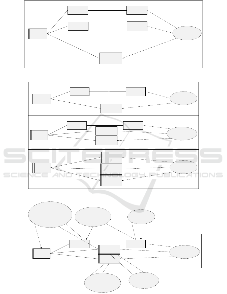
Step 2: Make Six Variables Explicit. The problem
diagram in Figure 6 shows the six variables for the
goal G2. G2 is formulated in active voice to repre-
sent the requirement in the problem diagram. The
machine that is developed is the ACC software. There
are two real world domains that are relevant and need
to be considered to satisfy the requirement: vehicles
ahead and the ACC vehicle itself. The following pro-
perties of these two problem domains need to be ob-
served and represent therefore referenced variables:
lane, speed, and distance of vehicles ahead as well
as lane and speed of the ACC vehicle. In order to
enable observation of these phenomena, the following
sensors have been chosen as solutions: a long range
radar sensor and ESP (Electronic Stability Program)
sensors. These sensors are not able to monitor the
referenced variables exactly, but they can be used to
make estimations of them. The relative position of
vehicles ahead represents, for example, an estimation
of their lane, and course of the ACC vehicle repre-
sents an estimation of its lane. These are annotated
in the problem diagram as monitored variables. The
ICSOFT 2018 - 13th International Conference on Software Technologies
106

estimation is done as follows: the long range radar
sensor detects vehicles ahead and is able to provide
data about their lateral offset, speed, and distance (in-
put data to the ACC software). ESP sensors provide
data about the ACC vehicle’s yaw rate, lateral accele-
ration, wheel speed, and steering wheel angle (input
data to ACC software). Based on the data from the
ESP sensors, the ACC software is able to predict the
course of the ACC vehicle. Based on the course of the
ACC vehicle and the lateral offset of vehicles ahead,
the ACC software is able to calculate the relative posi-
tion of vehicles ahead and thus to estimate whether a
vehicle ahead is driving on the same lane as the ACC
vehicle or not. Speed and distance of these vehicles
is stored (shown as the designed domain
2
‘Identified
vehicles ahead on same lane’). This data is then used
in the problem diagram of G3 (not shown here).
Step 3: Decompose Problem Diagram based on Re-
ferenced and Desired Phenomena. G2 was too com-
plex and therefore we decomposed it first according
to its referenced and desired phenomena into the fol-
lowing subgoals: G2.1: ‘Determine lane and speed of
ACC vehicle’, G2.2: ‘Determine lane, speed, and dis-
tance of vehicles ahead’, G2.3: ‘Determine vehicles
ahead on same lane’. The refined problem diagrams
are shown in Figure 7. In the first problem diagram,
the course of the ACC vehicle is calculated. In the se-
cond problem diagram, the relative position of vehi-
cles ahead is calculated. And finally, in the third pro-
blem diagram, both are compared to determine which
detected vehicle ahead is driving on the same lane as
the ACC vehicle. In case of G1 and G3 it was not
necessary to decompose them further. For these two
goals, we proceeded with Step 4.
Step 4: Make Assumptions and Software Require-
ments Explicit. Figure 8 shows the expectations, dom-
ain hypothesis, and software requirement for goal
G2.2. The problem diagram shows how lane, speed,
and distance of vehicles ahead are determined. These
are the variables of vehicles ahead that need to be ob-
served. Speed and distance are measured by the long
range radar sensor. The lane is estimated by means of
calculating the relative position of vehicles ahead. For
this calculation, the measured lateral offset is required
as well as the calculated course of the ACC vehicle.
Speed, distance, and relative position are then stored
in the model domain ‘Model of vehicles ahead’.
Since the monitored variable ‘relative position’ is
different from the referenced variable ‘lane’, there is a
2
A designed domain is a domain which is actually part
of the machine domain. The machine is typically consi-
dered as a black box. However, sometimes it is necessary
to model, for example, certain data stores. These are then
shown in problem diagrams as designed domains.
domain hypothesis DH-3 expressing that the relative
position should reflect the lane of vehicles ahead. Re-
garding the long range radar, we have the expectation
(Exp-LRR) that the measured data reflects correspon-
ding real world data. The ACC software has the task
to calculate the relative position based on the data it
receives from the long range radar sensor and the cal-
culated course (SofReq2). There are two model dom-
ains in the problem diagram. As explained above, we
expect that the modelled data reflects real world data
(DH-2 and DH-4).
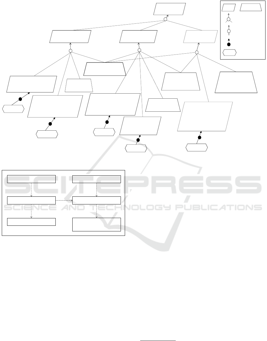
Step 5: Enhance KAOS Goal Model. Figure 9 shows
an excerpt of the extended KAOS goal model for the
ACC example. The excerpt focusses on the decom-
position of G2. A major advantage of our method is
that several domain hypotheses become explicit that
might otherwise (without a systematic approach like
ours) would have been neglected. The goal tree shows
also which interdependencies exist between the goals.
DH-2, for example, has a key role since it needs to be
valid for G2.1, G2.2, and G2.3. DH-4 also needs to
be valid for G2.2 and G2.3.
Step 6: Document Phenomena Dependencies. The
phenomena dependencies are shown in Figure 10.
The referenced variable ‘lane’ of vehicles ahead de-
pends on the monitored variable ‘relative position’.
Relative position depends on the measured lateral off-
set as well as the calculated course of the ACC vehi-
cle. And the calculated course depends on the me-
asured yaw rate, lateral acceleration, steering wheel
angle, wheel speed measured by the ESP sensors.
The benefit of the phenomena dependency dia-
gram is that changes are better manageable. Imagine
that the decision is made not to use the data from ESP
sensors any more. An impact analysis would proceed
in the following way. The goal model in Figure 9
shows that we have one expectation to be satisfied by
ESP sensors (Exp-ESPS). This expectation would not
be satisfied any more and this has a negative impact
on the satisfaction of the parent goal G2.1. In the pro-
blem diagram for G2.1 (Figure 7), the problem dom-
ain ‘ESP sensors’ and its two interfaces to ACC soft-
ware and to ACC vehicle would have to be deleted
from the diagram. However, an analysis of the phe-
nomena dependency diagram (Figure 10) reveals that
several other phenomena would be affected as well,
since they depend on the data from the ESP sensors,
namely: course of ACC vehicle, and in turn lane of
ACC vehicle, relative position of vehicles ahead, and
in turn lane of vehicles ahead.
Supporting the Systematic Goal Refinement in KAOS using the Six-Variable Model
107
ACC
Software
Vehicles
ahead
G2: Identify
vehicles ahead
on same lane
Identified
vehicles ahead
on same lane
ESP Sensors
Long Range
Radar
VA! {lane, speed,
distance}
VA! {relative position,
speed, distance}
LRR! {measured lateral
offset, speed, distance}
ACC vehicle
ACCV! {course,
current speed}
ESPS! {measured yaw rate, lateral acceleration,
wheel speed, steering wheel angle}
ACCV! {lane,
current speed}
IVAS! {speed, distance}ACC! {speed, distance of IVAS}
Figure 6: Six variables for goal G2.
ACC
Software
G2.1:
Determine
lane, speed, of
ACCV
Model of
ACC vehicle
ESP Sensors
ACC vehicle
ACCV! {course,
current speed}
ESPS! {measured yaw rate, lateral acceleration,
wheel speed, steering wheel angle}
ACCV! {lane,
current speed}
MACCV! {course, speed}
ACC! {course, speed}
ACC
Software
Vehicles
ahead
G2.2: Determine
lane, speed,
distance of VA
Model of
vehicles ahead
Long Range
Radar
VA! {lane, speed,
distance}
VA! {relative position,
speed, distance}
LRR! {measured lateral
offset, speed, distance}
MVA! {relative position, speed, distance}ACC! {relative position, speed, distance of MVA}
Model of
ACC vehicle
MACCV! {course}
MACCV! {course}
ACC
Software
G2.3:
Determine VA
on same lane
Identified
vehicles ahead
on same lane
IVAS! {speed, distance}
ACC! {speed, distance}
Model of
vehicles ahead
Model of
ACC vehicle
MVA! {relative position, speed, distance}
MACCV! {course, speed}
MVA! {relative position, speed, distance}
MACCV! {course, speed}
Figure 7: Decomposition of G2.
ACC
Software
Vehicles
ahead
G2.2: Determine
lane, speed,
distance of VA
Model of
vehicles ahead
Long Range
Radar
VA! {lane, speed,
distance}
VA! {relative position,
speed, distance}
LRR! {measured lateral
offset, speed, distance}
MVA! {relative position, speed, distance}ACC! {relative position, speed, distance of MVA}
Model of
ACC vehicle
MACCV! {course}
MACCV! {course}
DH-3: Relative
position of VA
reflects its
lane.
Exp-LRR: Measured
lateral offset, speed,
distance reflect corr.
values in real world.
SofReq2: Calculate
relative position based
on data from LRR and
calculated course and
store relative position,
speed, distance of VA.
DH-4: Calculated
relative position
reflects relative
position in real
world.
DH-2:
Calculated course
reflects course in
real world.
Figure 8: Relations between six variables for G2.2.
ICSOFT 2018 - 13th International Conference on Software Technologies
108
G2: Vehicle
ahead on same
lane identified
G2.2: Lane, speed,
distance of vehicle
ahead determined
G2.3: Vehicles
ahead on same
lane determined
G2.1: Lane, current
speed of ACC vehicle
determined
Exp-ESPS: Measured yaw
rate, lateral acc., wheel
speed, steering wheel angle
reflect corr. values in real
world.
DH-1: Course of
ACCV reflects its
lane.
SofReq1: Calculate course
based on data from ESPS
and store calculated
course and speed of ACCV
Exp-LRR: Measured
lateral offset, speed,
distance reflect corr.
values in real world.
SofReq2: Calculate relative
position based on data from
LRR and calculated course
and store relative position,
speed, distance of VA.
SofReq3: Compare course
of ACCV and relative
position of VA and
determine which VA is
driving on same lane, and
store speed and distance
of VA on same lane.
ACC
ESPS
ACC
LRR
ACC
responsibility
assignment
agent
goal
AND-refinement
OR-refinement
DH-2: Calculated course
reflects course in real
world.
DH-3: Relative
position of VA
reflects its lane.
DH-4: Calculated
relative position
reflects relative
position in real world.
DH-5: Identified
vehicles ahead on same
lane reflect vehicles
ahead on same lane in
real world.
domain
hypothesis
Figure 9: Enhanced KAOS goal model.
VA! {lane}
VA! {relative position}
LRR! {measured lateral offset}
depends on
depends on
ACCV! {lane}
ACCV! {course}
ESPS! {measured yaw rate,
lateral acceleration, steering
wheel angle, wheel speed}
depends on
depends on
depends on
Phenomena Dependency Diagram
Figure 10: Phenomena dependency diagram.
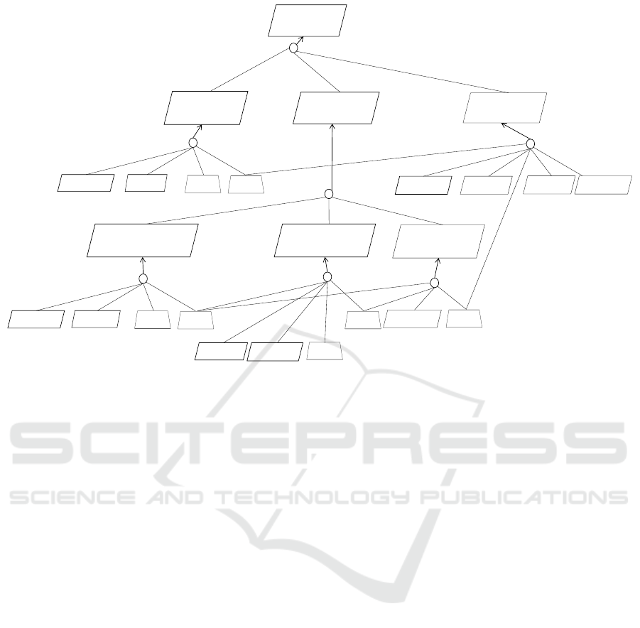
3.3 Benefit of Our Method
The benefit of our method is that domain hypotheses,
expectations, and software requirements are made ex-
plicit in a systematic way. In Figure 11, the complete
KAOS goal model is shown, i.e. the decomposition
of G0. Interestingly, the model shows that there are
interrelations between the decompositions of G1, G2,
and G3. Some domain hypotheses contribute to the
satisfaction of several goals. For example, DH-2 has
a central role since it contributes to the satisfaction of
G2.1, G2.2, and G2.3. Or, DH-5 contributes not only
to the satisfaction of G2.3 but also to the satisfaction
of G3. Without a systematic approach (as suggested
by our method), which guides developers in making
domain hypotheses and expectations explicit, it would
be quite hard to identify all these domain hypotheses.
Without the domain hypotheses, the subtrees of G1,
G2, and G3 would be fairly independent of each ot-
her.
Domain hypotheses are frequently neglected and
taken for granted. In the past, wrong and invalid dom-
ain hypotheses have resulted in several catastrophic
incidents including injuries and loss of life (see (van
Lamsweerde, 2009) for more details). Our method
supports developers in making all their domain hypot-
heses and expectations explicit, even if they sound tri-
vial at first sight. However, each domain hypothesis
and expectation must be considered during obstacle
analysis
3
to identify obstacles
4
to them and possible
causes of these obstacles. The causes are usually not
trivial but very realistic, and then corresponding coun-
termeasures can be taken. DH-1 and DH-3 (Figure 9)
could, for example, be obstructed, if the ACC vehicle
and the vehicle ahead are driving in a curve and are
both driving very close to the road marking separating
their two lanes. In such a case, the lane of the vehicle
ahead estimated by the ACC software could be wrong,
i.e. the ACC software could ‘assume’ that the vehicle
ahead is driving on the same lane although it is not.
The likelihood and criticality of such an obstacle has
to be assessed during obstacle analysis. This is only
3
An obstacle analysis is a kind of what-could-go-wrong
analysis; see (van Lamsweerde, 2009) for more details.
4
Obstacles are undesirable conditions that may become
true and then obstruct the satisfaction of goals (van Lam-
sweerde, 2009).
Supporting the Systematic Goal Refinement in KAOS using the Six-Variable Model
109
G2: Vehicle
ahead on same
lane identified
G2.2: Lane, speed,
distance of vehicle
ahead determined
G2.3: Vehicles
ahead on same
lane determined
G2.1: Lane, current
speed of ACC vehicle
determined
Exp-ESPS DH-1
SofReq1
DH-2
Exp-LRR
DH-3
SofReq2
DH-4
SofReq3
DH-5
G0: Desired
speed
maintained
G1: Desired
speed entered
G3: Speed
controlled
Exp-UI
DH-6
SofReq4
DH-7
Exp-EMS
SofReq5 Exp-ESP
Exp-ACCV
Figure 11: Complete KAOS goal model.
possible, when such fundamental domain hypotheses
have been made explicit.
4 RELATED WORK
Bleistein et al. (Bleistein et al., 2004) suggest a met-
hod for integrating problem diagrams and goal mo-
dels in general. They state that although requirements
refinement is supported in Jackson’s problem frames
approach (Jackson, 2001) by the paradigm of problem
progression, there is no direct linkage between the re-
quirements on higher levels and the ones on lower le-
vels. Goal models are useful to describe these explicit
linkages. Therefore, they combine the two approa-
ches. We use the same idea in our method. However,
the focus of Bleistein et al. is mainly on the refine-
ment of the requirement in problem diagrams and in
goal models, while we pay additionally much atten-
tion to making expectations and, especially, domain
hypotheses explicit.
Gol Mohammadi et al. (Mohammadi et al., 2013)
also suggest a method for combining problem di-
agrams and goal models. However, in contrast to
Bleistein et al., the requirement in the problem dia-
gram does not represent the goal from the goal model.
Instead, the goal is annotated in the problem diagram
and linked to the requirement therein. This expres-
ses that the satisfaction of the requirement contributes
to the satisfaction of the goal. The focus of Gol Mo-
hammadi et al. is also mainly on the refinement of
requirements. They do not consider expectations and
domain hypotheses.
Dao et al. (Dao et al., 2011) make a first at-
tempt towards considering assumptions. They cri-
ticize that many existing approaches do not consi-
der the issue of inadequate or insufficient domain as-
sumptions. Therefore, they suggest a new type of
model which is called domain concern model. Dom-
ain concerns are unexpected problems which might
occur because domain assumptions are not analysed
adequately and sufficiently (e.g. sensor malfunction,
power failure, motor malfunction, fire). They are mo-
delled as a feature tree in the domain concern model.
Beside the domain concern model, problem diagrams
and quality attribute models (i.e. goal models) are cre-
ated. Between the elements of these three types of
models, different types of relationships may be mo-
delled. For example, a domain concern may influence
a quality attribute (e.g. safety) negatively. Domains in
the problem diagram may influence domain concerns
and quality attributes positively or negatively. By mo-
delling these relationships, the impact of the design
(shown in the problem diagram) and the domain con-
cerns (in the domain concern model) on the quality
attributes becomes visible. This facilitates making
changes to the system design to improve achieving the
desired quality attributes. Although Dao et al. speak
about domain assumptions, they do not make them
explicit in the way we do it in our method in terms
ICSOFT 2018 - 13th International Conference on Software Technologies
110

of expectations and domain hypotheses. They simply
model problem domains and phenomena in the pro-
blem diagrams and call these domain assumptions.
Han et al. (Han et al., 2017) integrate KAOS goal
models and problem diagrams. However, their focus
is on self-adaptive cyber-physical systems. In contrast
to the other existing approaches described above, they
integrate KAOS goal models and problem diagrams
into one model and therefore suggest a new diagram
type called Adapt-Requirement Diagram. This dia-
gram shows not only the functional requirements (as
traditional problem diagrams do) but also the adapta-
tion requirements related to them. Thus, it has two
parts: one showing the problem context for achieving
the functional goal and one showing the problem con-
text for achieving the adaptation goal. The diagrams
contain elements of KAOS goal models (e.g. goals,
tasks, and AND/OR refinements), elements of pro-
blem diagrams (machine and problem domains, inter-
faces and requirement references) as well as new ele-
ments for expressing adaptation requirements (adap-
tation domains and ‘aggregate’ relationships). Since
self-adaptation is the ability of a system to adapt auto-
nomously to changes in its context/environment, Han
et al. consider a certain type of assumptions. Howe-
ver, these are dynamic assumptions that can be mo-
nitored at runtime. Our focus is on another type of
assumptions which are implicitly made by developers
during development of a software, are rather static,
and represent tacit knowledge.
5 CONCLUSION
In literature, several approaches can be found that
suggest integrating goal models and problem dia-
grams. The combination is fruitful because (i) both
can be used for defining requirements on different ab-
straction levels, (ii) problem diagrams show the pro-
blem context of each requirement, and (iii) goal mo-
dels show the direct links between higher level and lo-
wer level requirements. However, as we have shown
in this paper, the combination is not only beneficial
as regards requirements but also as regards assump-
tions. Since KAOS is the only goal modelling lan-
guage that supports the consideration of assumptions
(expectations and domain hypotheses) and is based on
the satisfaction argument, we have chosen this goal
modelling language for integration with problem di-
agrams. However, other goal modelling languages
may also be used instead of KAOS as long as they
show satisfaction relationships between super goals
and subgoals. Then they can be extended with con-
cepts for representing expectations and domain hypot-
heses. Many goal modelling approaches have already
been extended to allow for modelling some type of
assumptions.
In future work, we plan to carry out an empirical
evaluation focussing on the actual benefits of our in-
tegrated model in terms of required time and effort
for creating it as well as in terms of advantages for
developers.
REFERENCES
Bleistein, S., Cox, K., and Verner, J. (2004). Requirements
engineering for e-business systems: Integrating jack-
son problem diagrams with goal modelling and bpm.
In Proc. of APSEC 2004, pages 410–417. IEEE Com-
puter Society.
Dao, T., Lee, H., and Kang, K. (2011). Problem frames-
based approach to achieving quality attributes in soft-
ware product line engineering. In Proc. of SPLC 2011,
pages 175–180. IEEE Computer Society.
Han, D., Xing, J., Yang, Q., Li, J., Zhang, X., and Chen,
Y. (2017). Integrating goal models and problem fra-
mes for requirements analysis of self-adaptive cps.
In Proc. of COMPSAC 2017, pages 529–535. IEEE
Computer Society.
Jackson, M. (2001). Problem Frames - Analysing and Struc-
turing Software Development Problems. Addison-
Wesley.
Mohammadi, N. G., Alebrahim, A., Weyer, T., Heisel, M.,
and Pohl, K. (2013). A framework for combining
problem frames and goal models to support context
analysis during requirements engineering. In Proc. of
CD-ARES 2013, volume LNCS 8127, pages 272–288.
Springer.
Parnas, D. and Madey, J. (1995). Functional documents
for computer systems. Science of Computer Program-
ming, 25(1):41–61.
Ulfat-Bunyadi, N., Meis, R., and Heisel, M. (2016). The
six-variable model - context modelling enabling sys-
tematic reuse of control software. In Proceedings of
the 11th International Joint Conference on Software
Technologies, pages 15–26.
van Lamsweerde, A. (2009). Requirements Engineering -
From System Goals to UML Models to Software Spe-
cifications. John Wiley and Sons.
Zave, P. and Jackson, M. (1997). Four dark corners of requi-
rements engineering. ACM Transactions on Software
Engineering and Methodology, 6(1):1–30.
Supporting the Systematic Goal Refinement in KAOS using the Six-Variable Model
111
