A Simultaneous Cyber-attack and a Missile Attack
Bao U. Nguyen
Defence Research Development Canada, 101 Colonel By Drive, Ottawa, Canada
School of Mathematics and Statistics, University of Ottawa, 585 King Edward Avenue, Ottawa, Canada
Keywords: Cyber Defence, Missile Defence, Epidemic Models, Differential Equations, Probabilistic Models.
Abstract: We model a missile defence scenario where the red force infects the blue force command and control
systems while at the same time launching re-entry vehicles toward the blue force. As a result, the blue force
missile defence system is weakened due to loss of time, loss of engagement opportunities, loss of network
centric capabilities etc. The impacts of the cyber-attack on missile defence metrics are determined through a
number of key measures of effectiveness such as the probability of raid negation and the expected number
of targets neutralized.
1 INTRODUCTION
In a traditional missile defence scenario, a number of
re-entry vehicles (RVs) are launched toward a target.
In response, the defence engages the threats with
interceptors. Typically, such a scenario is analysed
with the number of engagement opportunities and an
engagement tactic to determine the metrics for
missile defence such as the probability of raid
annihilation,
PRA
, i.e. the probability of neutralizing
all RVs.
With the advent of cyber technologies, the red
force (the attacker) could also launch a cyber-attack
at the same time as a missile attack or shortly before.
This could lead the blue force (the defender) to lose
precious time to counter the RVs, or to lose
engagement opportunities, or to disable the defence
net centric capabilities or to completely incapacitate
the defence.
In this paper, we will model the cyber defence of
the blue force through an epidemic model known as
the SIR (Susceptible – Infected – Removed units)
model (Smith?, 2008). There are of course other
epidemic models e.g. Bailey, 1975, Hethcote, 2000
and Keeling and Rohani, 2007. However, we feel
that the SIR model has a suitable level of details for
this analysis. Morris-King and Cam, 2015 and Zou
et al., 2002 have also made use of epidemic models
to investigate cyber vulnerabilities. The SIR model
is described by three coupled differential equations.
Among the simple epidemic models, this is the first
that is not trivial and has no (elementary) known
analytical solution. However, we were able to derive
a relatively accurate analytical solution which is
used to determine the time evolution of the SIR
units. With this analytical solution, we estimate the
impact of a cyber-attack on
PRA
and other metrics.
2 THE SIR MODEL
The premise of the SIR model is encoded in the
following differential equations:
dS
aSI
dt
dI
aSI bI
dt
dR
bI
dt



(1)
where
S
is the number of susceptible units,
I
is the
number of infected unit and
R
is the number of
removed units i.e. the number of units that were
infected and then recovered;
a
is the rate of
infection and
b
is the rate of recovery.
Given that a missile attack lasts only a short time
(approximately less than an hour), it is consistent
with the SIR model that the population is a constant
i.e. we assume that there is not sufficient time to add
or remove new units. That is,
S I R N  
.
Therefore, it is convenient to scale the SIR units so
that the total population is one:
Nguyen, B.
A Simultaneous Cyber-attack and a Missile Attack.
DOI: 10.5220/0006847504930499
In Proceedings of 8th International Conference on Simulation and Modeling Methodologies, Technologies and Applications (SIMULTECH 2018), pages 493-499
ISBN: 978-989-758-323-0
Copyright © 2018 by SCITEPRESS – Science and Technology Publications, Lda. All rights reserved
493

' ' ' / 1S I R N N   
where
'/S S N
,
'/I I N
,
'/R R N
. For
convenience, we refer to
'S
as
S
,
'I
as
I
and
'R
as
R
. Harko et al., 2014 do provide a solution that
is very sophisticated. Here, we favour a more simple
approach that gives a simple solution.
Smith?, 2008 indicates that there are two
equilibrium points. The first occurs when
0II
,
S S N
and
R R N S  
(the upper bar refers
to the equilibrium values). This makes
/0dI dt 
.
Hence, there is no infection. And the second occurs
when
0aS b
or
/S S b a
which also
implies that
/0dI dt 
which makes
IIN
but
S
is decreasing due to
/dS dt
. Hence, this is not a
stable equilibrium.
However, if
0
/S b a
, the initial value of
S
at
time zero will lead to an epidemic as the number of
infected units
I
will increase with time at time zero
since
/0dI dt 
.
Nguyen, 2017 shows that to solve the SIR model
is equivalent to solve the following differential
equation:
0
1
af
df
bf S e
dt

  
(2)
where
   
0
0
t
f t I t dt

(3)
with boundary conditions:
   
 
 
0
0
0
0
00
0
00
0
0
1
0
f I t dt
df
II
dt
SS
SI
R






(4)
In addition, there are two roots (Mathematica
2011) to the RHS of Eqn (2):
/
0
1
/
0
2
11
1,
11
0,
ab
ab
aS
f f W e
b a b
aS
f f W e
b a b




   




  


(5)
with
W
the Lambert functions. For a real argument
x
, there are two branches to the Lambert functions:
 
1,Wx
and
 
0,Wx
, Mathematica, 2011. Based
on the characteristics of the Lambert function,
Nguyen, 2017 shows that
2
0f 
and
1
0f 
.
Nguyen, 2017 also shows that the RHS of Eqn (2) is
a convex function in
f
. This leads to an
approximation of the RHS of Eqn (2) as a quadratic
function:
  
12
1
af
bf e c f f f f

   
(6)
While Eqn (6) captures the convexity of Eqn (2),
Eqn (6) does not reproduce the asymmetry of Eqn
(2). This is so as a quadratic function in
f
is a
symmetrical function with respect to its vertex
 
 
12
/2f f f
. Therefore, we propose an
improvement to this approximation.
3 NEW APPROXIMATION TO
THE SIR MODEL
As a correction to Eqn (6), we introduce a parameter

such that
   
11
12
1
af
bf e c f f f f
 

   
(7)

is chosen so that the LHS and the RHS of Eqn (7)
match at
 
0
*
ln /a S b
ff
a


where the LHS of
Eqn (7) is a maximum.
Since the LHS of Eqn (7) is a convex function,
this is the only maximum. Hence, there is no
ambiguity in determining

:
 
*
12
12
/2f f f
ff




(8)
Figure 1:
/df dt
from Eqn (2), quadratic approximation
in Eqn (6) and asymmetric approximation Eqn (7) – (
1/ 2a 
,
1/ 3b 
,
0
0.99S 
,
0
0.01I 
and
0
0R 
).
0
0,02
0,04
0,06
0,08
0,1
0 0,5 1 1,5 2
df/dt
f
df/dt as a function of f
Exact
Quadratic
Asymmetric
DMSS 2018 - Defence and Military
494

Figure 2:
/df dt
from Eqn (2), quadratic approximation
in Eqn (6) and asymmetric approximation Eqn (7) – (
3/ 2a 
,
1/ 3b 
,
0
0.99S 
,
0
0.01I 
and
0
0R 
).
Figure 1 shows
/df dt
as a function of
f
for
three cases: the exact case, the quadratic
approximation and the asymmetric approximation.
We assume that
1/ 2a 
,
1/ 3b 
,
0
0.99S 
,
0
0.01I 
and
0
0R 
. It can be seen that the three
cases are similar.
Figure 2 also shows
/df dt
as a function of
f
for three cases: the exact case, the quadratic
approximation and the asymmetric approximation.
We assume that
3/ 2a 
,
1/ 3b 
,
0
0.99S 
,
0
0.01I 
and
0
0R 
. It can be seen that the
quadratic approximation is distinct from the two
other cases.
Note that the values of the above parameters --
a
,
b
,
0
S
,
0
I
and
0
R
-- were used for illustration
purposes only.
Using the approximation on the RHS of Eqn (7),
i.e.
   
11
12
df
c f f f f
dt
 
  
(9)
or
   
11
12
df
dt
c f f f f
 


We obtain:
   
 
12
21
1
f f f f
tA
c f f



  
  

Since
0f 
when
0t 
, we get:
 
1
2 2 1
11
f
A
c f f f




  



(10)
Matching Eqn (7) at
*
ff
dictates that:
 
 
   
0
11
**
12
1 / 1 ln /b a a S b
c
f f f f
 
   

  
(11)
Now that all of the parameters are well defined,
we could solve Eqn (9):
21
2
1
ff
ff
u



(12)
where
   
1/
21
u c f f t A

      


(13)
Since
/I df dt
, we get:
 
 
2
1
21
2
1
c f f u
I
u
 
  


(14)
By manipulating Eqn (1), Nguyen, 2017 shows
that:
 
0
a f t
S S e


(15)
and
 
R b f t
(16)
4 PROPERTIES OF THE
APPROXIMATION
The maximum of
I
occurs when
/0dI dt 
. Using
Eqn (14), we get:
 
 
 
1
*
2
max 2 1
2
*
1
u
I c f f
u
 
   

(17)
where
*
1
1
u





(18)
This corresponds to
0
0,1
0,2
0,3
0,4
0,5
0 1 2 3
df/dt
f
df/dt as a function of f
Exact
Quadratic
Asymmetric
A Simultaneous Cyber-attack and a Missile Attack
495

 
*
*
u
tA
c




(19)
Taking the limit as
t 
of Eqn (14) yields:
lim 0
t
I


(20)
Similarly,
2
lim
t
ff


(21)
Therefore,
2
0
lim
af
t
S S e



(22)
and
2
lim
t
R b f


(23)
Note that by taking the limit
0  
, we recover
the results of Nguyen 2017 i.e.
 
21
1
0
2
lim
c f f t
f
ue
f

  






(24)
We display below
S
,
I
and
R
as a function of
time. The exact case is obtained numerically using
Mathematica, 2011.
Note that we could also determine the time when
I
decreases to a small amount

after it reaches the
maximum value. That is,
 
 
2
1
21
2
1
c f f u
I
u



  


(25)
or
 
2
1
'1uu



  
(26)
where
 
2
21
'
c f f

 

(27)
We use perturbation theory to get the first order
approximation for
 
2
01
u u u O     
by
expanding Eqn (26) as a series in powers of

. By
carefully the value of
u
that occurs after the
maximum of
I
, we get:
 
0
1 2 ' 1 4 ' 1
2'
2 ' '
uO



    
   

(28)
and
 
0
1 2 ' 1 4 ' 1
2'
2 ' '
uO



    
   

(29)
 
 
 
 
00
1
0
ln ln '
2'
1 2 ' 1 '
uu
uO
u




   
   
(30)
Hence,
 
 
2
01
u u O
tA
c



  


(31)
This works for very small values of

and very
small values of
' 
. An alternative, accurate and
efficient way to determine the time is to use the
rigorous bisection methodology in Press et al. 1992
where would be bracketed in the interval:
0
1
1,
'
u





(32)
The corresponding time can be determined in a
similar way to Eqn (19) (without the
*
).
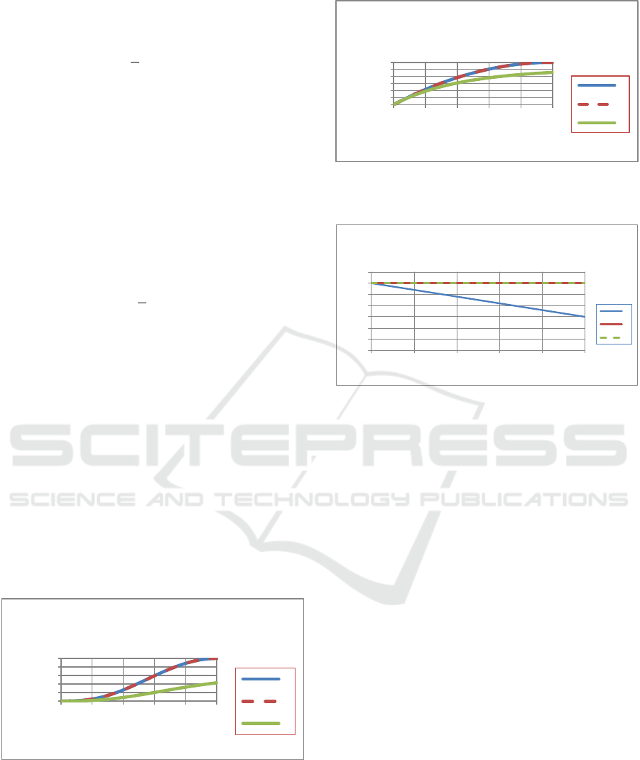
Figures 3, 4 and 5 show that the approximations
reproduce the characteristics of the exact numerical
solution.
S
decreases monotonically as a function
of time.
I
increases and then decreases as a
function of time.
R
increases monotonically as a
function of time. The asymmetric approximation is
clearly closer to the exact solution than the quadratic
approximation. More importantly, the asymmetric
approximation replicates the asymmetry of
/df dt
which is essential to the SIR model since there is no
reason for the independent parameters
a
and
b
to
combine in a way such that
/df dt
is symmetric in
f
.
Figure 3:
S
as a function of time for the exact case, the
quadratic approximation and the asymmetric
approximation.
0
0,2
0,4
0,6
0,8
1
0 10 20 30 40
S
Time
S as a function of time
Exact
Quadratic
Asymmetric
DMSS 2018 - Defence and Military
496

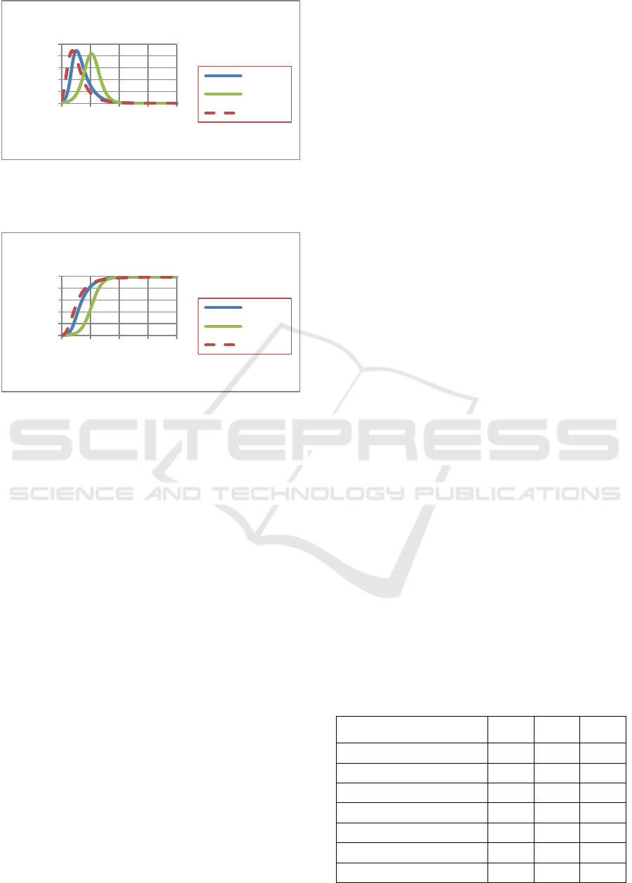
Figure 4:
I
as a function of time for the exact case, the
quadratic approximation and the asymmetric
approximation.
Figure 5:
R
as a function of time for the exact case, the
quadratic approximation and the asymmetric
approximation.
5 EFFECTS ON MISSILE
DEFENCE
To examine the impacts of infection on missile
defence capabilities, we consider a scenario where
there are three re-entry vehicles (RVs) and six
interceptors. We assume that there are two
engagement opportunities.
Normally, given the speeds and ranges involved
Cranford, 2004 could be used to determine the
number of engagement opportunities for ballistic
missile trajectories. The key metrics are the
probability of raid annihilation
 
PRA
-- the
probability of neutralizing all RVs, the expected
number of RVs neutralized
 
ERVN
and the
expected number of interceptors expended
 
ENIE
.
These metrics are parametrized by the single shot
probability of a hit
H
.
When the defence is infected with viruses, the
missile defence capabilities could also be affected.
As shown in Figure 4, it takes the defence about
twenty minutes to remove the infection. We consider
below three possible scenarios:
A. The defence is unaffected;
B. The defence loses one engagement
opportunity and
C. The defence loses its coordination such as
its network centric capabilities.
In scenario A, the defence uses a shoot-look-
shoot tactic. It engages each RV with one interceptor
at each engagement opportunity. If the RV is
neutralized then the defence will stop engaging that
RV. Otherwise, the defence will re-engage the RV
with another interceptor until the defence runs out of
interceptors or engagement opportunities. The
metrics for scenario A are given below.
 
3
2
1PRA M
(33)
 
2
31ERVN M  
(34)
33ENIE M  
(35)
where
1MH
.
In scenario B, the defence will launch all of its
interceptors at the second engagement opportunity.
This gives:
 
3
2
1PRA M
(36)
 
2
31ERVN M  
(37)
6ENIE 
(38)
In scenario C, the defence loses its coordination
hence it cannot allocate the interceptors optimally
among the RVs. The optimal allocation occurs when
the defence assigns the interceptors as evenly as
possible among the RVs, Soland, 1987, at each
engagement opportunity. The possible allocations
are determined in Nguyen and Miah, 2015 as shown
in Table 1.
Table 1: All possible engagement allocations against three
RVs.
Engagement allocation
RV 1
RV 2
RV 3
1
0
0
6
2
0
1
5
3
0
2
4
4
0
3
3
5
1
1
4
6
1
2
3
7 (Optimal Salvo tactic)
2
2
2
0
0,1
0,2
0,3
0,4
0,5
0 10 20 30 40
I
Time
I as a function of time
Exact
Quadratic
Asymmetric
0
0,2
0,4
0,6
0,8
1
0 10 20 30 40
R
Time
R as a function of time
Exact
Quadratic
Asymmetric
A Simultaneous Cyber-attack and a Missile Attack
497

Assuming that each allocation in Table 1 is
equally probable then
PRA
can be expressed as:
7
1
1
7
i
i
PRA p



(39)
where
1 2 3 4
, , , 0p p p p 
(40)
 
 
2
4
5
11p M M   
(41)
 
   
23
6
1 1 1p M M M     
(42)
 
3
2
7
1pM
(43)
As well,
ERVN
can be expressed as:
7
1
1
7
i
i
ERVN e



(44)
6
1
1eM
(45)
5
2
2e M M  
(46)
24
3
2e M M  
(47)
3
4
22eM  
(48)
4
5
32e M M   
(49)
23
6
3e M M M   
(50)
2
7
33eM  
(51)
Also,
ENIE
is given by:
6ENIE 
(52)
Figure 6:
PRA
as a function of the single shot probability
of a hit
.H
Figures 6, 7 and 8 plot the missile defence
metrics as a function of the single shot probability of
a hit
H
. It is seen that
PRA
and
ERVN
are the
same for scenario A and for scenario B. However,
Figure 7:
ERVN
as a function of the single shot
probability of a hit
.H
Figure 8:
ENIE
as a function of the single shot
probability of a hit
.H
they are substantially lower for scenario C. This is
due to the fact that in scenario C, the engagement
allocation is not optimal.
ENIE
is equal to six for scenario B and scenario
C but is decreasing as a function of
H
for scenario
A. This means that in scenario B and in scenario C,
the defence launches all of its interceptors. This is
very dangerous as the defence will not have any
interceptors left to engage unexpected RVs or to re-
engage RVs that were missed due to malfunctions of
the defence systems. For scenario A, with a typical
H
of seventy percent, Figure 8 shows that the
defence will have expended four interceptors
implying the defence will have two interceptors
remaining for unexpected events. As
H
increases,
ENIE
decreases and so the number of interceptors
saved increases.
We observe that when the number of RVs and
the number of interceptors are large, the metrics
such as
PRA
and
ERVN
can be efficiently
determined using a generating function e.g. Nguyen
et al., 1997. Missile defence can also be modelled
using Markov chains e.g. Menq et al., 2007 and
globally optimized using dynamic programming e.g.
Soland, 1987.
0
0,2
0,4
0,6
0,8
1
0 0,2 0,4 0,6 0,8 1
PRA
H
PRA as a function of the single shot
probability of a hit
A
B
C
0
0,5
1
1,5
2
2,5
3
0 0,2 0,4 0,6 0,8 1
ERVN
H
ERVN as a function of the single shot
probability of a hit
A
B
C
0
1
2
3
4
5
6
7
0 0.2 0.4 0.6 0.8 1
ENIE
H
ENIE as a function of the single shot
hit probability
A
B
C
DMSS 2018 - Defence and Military
498

6 CONCLUSIONS
In this paper, we examine a missile attack scenario
combined with a cyber-attack scenario. To do that,
we solve the SIR model using an approximate
solution which reproduces all of the characteristics
of the problem such as the asymmetry, the trends in
time evolution of the parameters
I
,
S
and
R
as well
as their long term behaviours.
It could also be argued that the asymmetric
approximation is in itself an epidemic model in the
same way that the SIR model is an epidemic model.
They are both anchored on similar assumptions. And
they both generate similar results.
We show that the missile defence effectiveness
of the blue force can be critically affected when the
red force launches a cyber-attack at the same time as
a missile attack.
To our knowledge, the degradations of a missile
defence system due to a cyber-attack have not been
explicitly modelled. In the future, we would like to
examine closely how command and control systems
are affected by a cyber-attack. To do that, we will
investigate in depth the complexity of command and
control systems and the nature of cyber-attacks.
REFERENCES
Bailey, N.T.J., 1975. The mathematical theory of
infectious diseases and its applications, Charles
Griffin and Company LTD, 2nd edition, pp. 39-42.
Cranford K.. 2004. Battle Area Region Threatened Model
(BART). NORAD-USNORTHCOM/AN (North
American Aerospace Defense Command – United
States Northern Command/Center for Aerospace
Analysis) Version 5.3.4x. and the CheckThreats
subroutine.
Harko, T., Lobo, F.S.N., and Mak, M.K., 2014. ‘Exact
analytical solutions of the Susceptible-Infected-
Recovered (SIR) epidemic model and of the SIR
model with equal death and birth rates’, Applied
Mathematics and Computation, 236, pp. 184-194.
Hethcote, H., 2000. ‘The mathematics of infectious
diseases’, SIAM Review, Vol. 42, No. 4, pp. 599-653.
Keeling, M.J. and Rohani, P., 2007. Modeling Infectious
Diseases in Humans and Animals, Princeton
University Press, p. 4.
Mathematica 2011. Wolfram Research Inc.
Menq J.-Y., Tuan P.-C. and Liu T.-S., 2007. ‘Discrete
Markov Ballistic Missile Defense System Modeling’,
European Journal of Operational Research, 178, pp.
560–578.
Morris-King, J. and Cam, H., 2015. ‘Ecology-inspired
cyber risk model for propagation of vulnerability
exploitation in tactical edge’, Proceedings of the IEEE
2015 Military Communications Conference
MILCOM'2015, pp. 336-341.
Nguyen B.U., Smith P.A. and Nguyen D., 1997. ‘An
Engagement Model to Optimize Defense Against a
Multiple Attack Assuming Perfect Kill Assessment’,
Naval Research Logistics, 44, pp. 687-697.
Nguyen, B.U., 2017. ‘Modelling cyber vulnerabilities
using epidemic models’, 7th international conference
on simulation and modelling methodologies,
technologies and applications.
Nguyen, B. and Miah, S., 2015. ‘Comparison of metrics
for missile defence between perfect coordination and
no coordination’, DRDC Scientific Report (SR)
DRDC-RDDC-2015-R228.
Press, W.H., Flannery, B.P., Teukolsky, S.A. and
Vetterling W.T., 1992. Numerical recipes in Fortran
77 (The Art of Scientific Computing). Cambridge
University Press, 2nd edition, pp. 343-347.
Smith? R., 2008. Modelling disease ecology with
mathematics, American Institute of Mathematical
Sciences, pp. 14-30.
Soland, R. M., 1987. ‘Optimal Terminal Defense Tactics
when Several Sequential Engagements Are Possible’,
Operations Research, 35, pp. 537-542.
Zou, C.C., Gong, W., and Towsley, D., 2002. Code red
worm propagation modeling and analysis,
Proceedings of the 9th ACM conference on Computer
and communications security, pp. 138-147.
A Simultaneous Cyber-attack and a Missile Attack
499