Path Tracking with Orthogonal Parametrization for a Satellite with
Partial State Information
Wojciech Domski and Alicja Mazur
Wrocław University of Science and Technology, Wrocław, Poland
Keywords:
Free-floating Satellite, Path Following, Object Capturing.
Abstract:
This article presents an orthogonal parametrization for a space robot. A simulation scenario was presented
where a satellite with a fixed 2R planar manipulator arm is chasing a moving object in the space. A path
tracking algorithm with partial state information such as distance to chased object and difference in orientation
was used. Due to the undemanding nature of proposed algorithm the satelite can successfully chase an object
with limited state information. The chase manoeuvre is divided into two stages. The first stage is to enter an
orbit around the object while following curvilinear path. In turn, the second stage is to settle in a point on the
orbit to create favourable conditions for any further operations.
1 INTRODUCTION
Space robotics is widely researched topic were vari-
ety of problems are still being solved i.e. trajectory
planning (Rybus and Seweryn, 2015). One of appli-
cations of space robots is debris removal (Kanazaki
et al., 2017), (Li et al., 2016). During the space mis-
sions a number of debris are left on Earth orbit. So-
metimes such debris are just leftovers and sometimes
those are parts of space object which were involved
in crash of various nature. The number of such space
litter is increasing and removing it is an emerging pro-
blem for sustaining safety of future missions. In this
article we propose an approach which allows a satel-
lite to chase other space objects and makes possible
further interaction with it. However, in space the in-
formation about state of chased object is limited and
sometimes it is very difficult to obtain relevant infor-
mation about the object’s state (Diaz and Abderrahim,
2006), (C. M. Allen et al., 2008). We have presented
an algorithm of path tracking problem with orthogo-
nal parametrization using Serret–Frenet description.
The Serret-Frenet frame was successfully used in path
following problem with marine vessels (Do and Pan,
2003). Undoubtedly, the biggest advantage of propo-
sed approach is the ability to work with limited in-
formation about the object. Two variables are requi-
red – a distance to chased object and its orientation
error. As discussed before, in contrast to other met-
hods which require a specific position and orientation
of chased object in global frame, our approach only
requires information about the distance to the object
and the orientation error. The distance between our
satellite and the object can be acquired with a laser
scanner while the orientation can be determined with
a camera system. In this work we consider a flat satel-
lite with 2 DoF robotic arm attached to the base with
offset.
In Section 2 mathematical model of satellite’s dy-
namics is presented. In turn, in Section 3 orthogonal
parametrization relative to Serret–Frenet frame is des-
cribed. Control problem and additional assumptions
are presented in Section 4. In Section 5 the control al-
gorithm has been introduced. The Section 6 presents
conducted simulations for flat satellite with manipu-
lating arm while Section 7 offers summary and dis-
cussion on obtained simulations.
2 MATHEMATICAL MODEL
In this article we will consider flat satellite, so-called
base, with manipulating arm. The satellite is made of
a rectangular shape where a rigid manipulator with
fixed two rotational joints is mounted. This object
moves on a plain with affiliated global coordination
system X
0
Y
0
Z
0
. The position of local coordination sy-
stem associated with centre of the mass of the satel-
lite’s base is X
b
Y
b
Z
b
.
Schematic of considered satellite and onboard ma-
nipulator is presented in Fig. 1.
252
Domski, W. and Mazur, A.
Path Tracking with Or thogonal Parametrization for a Satellite with Partial State Information.
DOI: 10.5220/0006835102520257
In Proceedings of the 15th International Conference on Informatics in Control, Automation and Robotics (ICINCO 2018) - Volume 2, pages 252-257
ISBN: 978-989-758-321-6
Copyright © 2018 by SCITEPRESS – Science and Technology Publications, Lda. All rights reserved

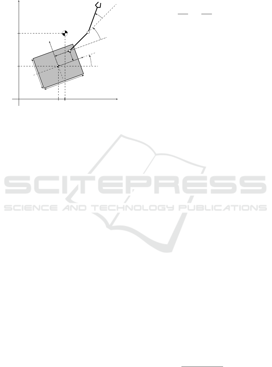
X
0
Y
0
w
h
X
b
Y
b
l
1
l
2
b
a
x
y
x
1e
x
2e
θ
q
1
q
2
Figure 1: Satellite with marked coordination systems.
2.1 Kinematics
Transformation from global coordination system to
satellite’s local coordination system can be expressed
as
A
b
0
= Trans(X,x)Trans(Y, y)Rot(Z, θ). (1)
Transformation from global coordination system to
the end of the first link can be written as
A
1
0
= A
b
0
Trans(X,a)Trans(Y, b)Rot(Z, q
1
)Trans(X,l
1
),
(2)
while the transformation from global coordinate sy-
stem to the end of the second link, so-called end-
effector, is described as
A
2
0
= A
1
0
Rot(Z,q
2
)Trans(X,l
2
). (3)
For further consideration we need the kinematics of
the end-effector including its position and orientation
relative to global frame. Finally, we can define kine-
matics of the end–effector as
k
e f
=


x
e f
y
e f
θ
e f


(4)
where:
x
e f
= x + a cos
θ
−b sin
θ
−l
1
(sin
1
sin
θ
−cos
1
cos
θ
)
−l
2
(cos
2
(sin
1
sin
θ
−cos
1
cos
θ
)
+sin
2
(cos
1
sin
θ
+cos
θ
sin
1
))
y
e f
= y + b cos
θ
+a sin
θ
+l
1
(cos
1
sin
θ
+cos
θ
sin
1
)
+l
2
(cos
2
(cos
1
sin
θ
+cos
θ
sin
1
)
−sin
2
(sin
1
sin
θ
−cos
1
cos
θ
))
θ
e f
= θ + q
1
+ q
2
.
Symbols have following meaning: sin
i
= sinq
i
and
cos
i
= cosq
i
, i = 1,2.
Calculating time derivative of k
e f
, we obtain
˙
k
e f
=
∂k
e f
∂q
b
˙q
b
+
∂k
e f
q
r
˙q
r
= J
b
˙q
b
+ J
r
˙q
r
(5)
where state vector q = (q
b
,q
r
)
T
: q
b
= (x,y, θ)
T
and
q
r
= (q
1
,q
2
)
T
.
2.2 Dynamics
Dynamics of the whole system was expressed in ge-
neralized coordinates. Satellite’s dynamics can be ex-
pressed in following equation (Siciliano and Khatib,
2007)
M ¨q +C = Bu, (6)
or more in detail as

M
b
M
bm
M
T
bm
M
m

¨q
b
¨q
r

+

c
b
c
r

=

B
b
0
0 0

u
0

, (7)
where M is inertia matrix, and c
b
and c
r
are other ele-
ments of dynamics related to Coriolis and centrifugal
forces of the base and of the manipulator arm. u is in-
put vector for controlling the thrusters which in turn
actuate the flat satellite and the B
b
is the input matrix.
It is assumed that the joint position of the manipu-
lator are fixed and do not change, thus the dynamics
regarding the acceleration of manipulator’s joint can
be omitted. As written above the manipulator joints
are fixed at initial position and do not move. This
condition is true during the whole phase of chasing
an object, as explained latter.
Another assumption was made for gravitation for-
ces, since the research object is in space it is influen-
ced by the micro-gravity and therefore the gravitation
force can be neglected. Also, as mentioned earlier,
the satellite’s base is actuated with three thrusters.
2.3 Thrusters Modelling
Moments generated by thrusters are present in local
coordination system of the satellite. However, to mo-
del those actuator the moments should be transformed
into global coordinate system. First vector of force for
i
th
thruster has to be decomposed into three elements:
an element which direction is aligned with X
b
axis of
the flat satellite coordinate system and with Y
b
axis.
The third element has to be perpendicular to the line
connecting the thruster mount point and the centre of
the mass of the satellite. For each thruster a vector of
three elements is calculated and then transformed to
the global coordination system. Those elements can
be expressed with following formulas:
v
x
= αcos(β) (8)
v
y
= αsin(β) (9)
v
θ
=
q
(1 − α
2
)(x
2
+ y
2
)sgn(sin(φ −β))(10)
Path Tracking with Orthogonal Parametrization for a Satellite with Partial State Information
253

where α = cos(φ − β), β = atan(
y
x
). x, y, φ are thrus-
ters position in X
b
axis, Y
B
axis and angle of mounting
thruster on the base in its local coordinate system re-
spectively. After calculation of all three elements (v
x
,
v
y
, v
θ
) for each thruster a matrix can be composed
where i
th
column holds three values calculated for i
th
thruster. This matrix is then transformed to the global
coordinate system with rotation matrix around Z axis.
The general form of control matrix B
b
is following:
B
b
=


v
x,1
v
x,2
v
x,n
v
y,1
v
y,2
··· v
y,n
v
θ,1
v
θ,2
v
θ,n


(11)
By choosing the placement, the orientation and
the number of thrusters on the satellite we can ensure
that the matrix is invertible. In the Section 6 place-
ment of the thrusters and its orientation was provided
and also the value of B matrix determinant.
3 ORTHOGONAL PATH
PARAMETRIZATION
In this paragraph we want to present specific descrip-
tion of the satellites’s motion – not relative to fixed
frame but relative to moving space debris.
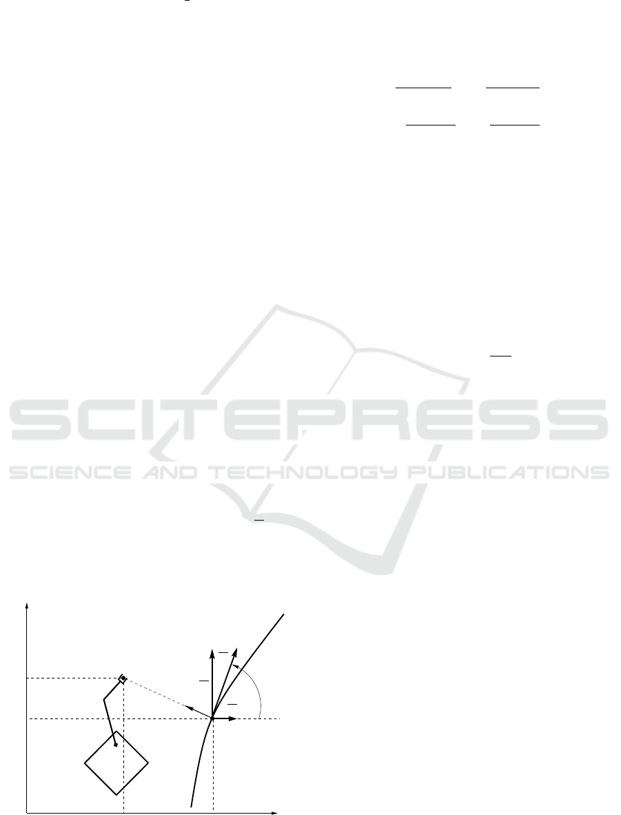
The path P is characterized by a curvature κ(s)
which is an inversion of the radius of the circle tangent
to the path at a point characterized by the parameter
s, see Fig. 2. We consider a moving point M and the
associated Serret-Frenet frame defined on the curve P
by the normal and tangent unit vectors x
n
and
dr
ds
. The
point M is any point, which should be tracked, e.g.
position of the end-effector in our case. In turn M’ is
the orthogonal projection of the point M on the path
P(s).
t
X
0
0
Y
x
n
r
2
θ
2
M
M’
s
P
x
y
r
1
dr
ds
ds
dr
l
1
dr
ds
Figure 2: Path P and projection of point M on the path P.
To describe the satellite’s motion relative to given
path we can use certain geometric relationships (Ma-
zur, 2004)
˙
l = −sin θ
t
˙x
e f
+ cosθ
t
˙y
e f
, (12)
˙
˜
θ =
κ(s)cos θ
t
κ(s)l − 1
˙x
e f
+
κ(s)sin θ
t
κ(s)l − 1
˙y
e f
+
˙
θ
e f
,(13)
˙s = −
cosθ
t
κ(s)l − 1
˙x
e f
−
sinθ
t
κ(s)l − 1
˙y
e f
. (14)
l is the distance between point on a path and the end–
effector,
˜
θ is the orientation error – it is a difference
between the orientation of the end–effector and the
orientation of the Serret-Frenet frame on the path.
Curvilinear distance s is a term which defines where
on the contour of the path the Serret-Frenet frame is
located.
Since the orthogonal parametrization is local
transformation the following conditions has to be ful-
filled during control (Fradkov et al., 1999)
r
min
> 0, (15)
κ(s) ≤
1
r
min
, (16)
l < r
min
. (17)
It means that the radius of any circle tangent to path
P(s) in two or more points has to be limited from be-
low with some positive number r
min
while interior of
such a circle can not contain any point which belongs
to the curve P(s). What is more, the distance l has
to be smaller then the minimal radius which in turn
yields that this parametrization is indeed local.
4 CONTROL PROBLEM
STATEMENT
The goal of the paper is to develop the control algo-
rithm for the flat satellite with onboard manipulating
arm, which allows to catch space debris with only par-
tial information about state of the object. The control
scheme will be divided into two steps:
1. Object tracking – motion of the base with immo-
bile manipulator realized with thrusters. After this
phase of motion satellite should be in the neig-
hbourhood of object, in such distance that it would
be possible to catch object only with manipula-
tor’s motion.
2. Object catching – near object the satellite should
stop, turn-off thrusters and try to catch the object.
This motion phase should be realized only with
manipulating arm.
ICINCO 2018 - 15th International Conference on Informatics in Control, Automation and Robotics
254

The information, which we have during the first
phase, is only partial – we don’t get information
about position relative to the global coordinate system
X
0
Y
0
Z
0
but we have only local information obtained
from sensors:
– shortest distance between satellite’s point M and
its orthogonal projection on object’s path M’,
– orientation error
˜
θ = θ − θ
t
– difference between
object’s and chaser satellite’s angle.
4.1 Assumptions
In this article we have taken the following assumpti-
ons:
• the motion of the tracked object and the chasing
satellite (chaser) is realized on the same plane
• the path, the object is moving along, is regular –
it can be approximated by the smooth flat curve
• dynamics of the chaser is fully known.
5 CONTROL ALGORITHM
As it has been mentioned in the previous section, the
control strategy contains two phases: tracking the
path of the object and reduction of the distance be-
tween the chaser and the object and, next, catching
the object with manipulating arm, if satellite is near
the object in reachable distance. However, in this pa-
per we have reduced our interest to design the control
method for the first phase.
5.1 Chasing the Object – Path
Following Problem
In the text we have written that chasing the object can
be treated as path following problem. For this reason
lets take satellite’s equations expressed relative to the
moving object (12)-(14) and rewrite them in the ma-
trix form
˙
ξ = Λ
˙
k
e f
, (18)
where path tracking variables are defined as follows
ξ =


l
˜
θ
s


, (19)
and matrix Λ equals to
Λ =



−sin θ
t
cosθ
t
0
κ(s)cos θ
t
κ(s)l−1
κ(s)sin θ
t
κ(s)l−1
1
−
cosθ
t
κ(s)l−1
−
sinθ
t
κ(s)l−1
0



. (20)
Matrix Λ is nonsingular as long as local parametriza-
tion is valid, i.e.
det Λ =
−1
κ(s)l − 1
6= 0 (21)
where fraction denominator is not equal to 0.
5.2 Decoupling and Linearization
To design a control algorithm based on orthogonal pa-
rametrization, we need to differentiate (18) with time
¨
ξ =
˙
Λ
˙
k
e f
+ Λ
¨
k
e f
. (22)
On the other hand we have assumed, that the joint
positions of the satellite’s manipulator are fixed and
do not move during path following process. It me-
ans that the dynamics (7) regarding the acceleration
of manipulator’s joint can be omitted, giving the sim-
plified form
M
b
¨q
b
+ c
b
= B
b
u. (23)
The condition treating about fixed joint is true during
the whole phase of chasing an object, therefore (5)
can be recalculated as follows
˙
k
e f
=
∂k
e f
∂q
b
˙q
b
= J
b
(q
b
) ˙q
b
(24)
with Jacobi matrix given below
J
b
=


1 0 −b cos
θ
−asin
θ
−l
2
sin
12θ
−l
1
sin
1θ
0 1 a cos
θ
−bsin
θ
+l
2
cos
12θ
+l
1
cos
1θ
0 0 1


Matrix J
b
is always invertible, because it holds
∀ q
b
∈ R
3
det J
b
(q
b
) = 1.
The term
¨
k
e f
can be obtained from equation (24)
¨
k
e f
=
˙
J
b
˙q
b
+ J
b
¨q
b
. (25)
Now, we put (25) into (22) and get
¨
ξ =
˙
Λ
˙
k
e f
+ Λ

˙
J
b
˙q
b
+ J
b
¨q
b

. (26)
The final step is to take into consideration dynamics
of the satellite.
After inserting dynamics (23) into the above equa-
tion we get affine control system
¨
ξ = F +Gu (27)
where F =
˙
Λ
˙
k
e f
+ Λ
˙
J
b
˙q
b
− ΛJ
b
M
−1
b
c
b
and G =
ΛJ
b
M
−1
b
B
b
.
It is easy to check that G matrix is invertible i.e. it
fulfils regularity condition detG 6= 0, because
G
−1
= B
−1
b
M
b
J
−1
b
Λ
−1
and every element in G
−1
is well defined and inverti-
ble.
Path Tracking with Orthogonal Parametrization for a Satellite with Partial State Information
255

Next we define control law for the system (27)
u = G
−1
(v − F), (28)
where v is a new input to the system. The closed-loop
system (27)-(28) is fully decoupled and linearised
¨
ξ = v, (29)
i.e. it is equivalent to the linear system of “double
integrator” type.
To control such system we propose PD-control
with compensation signal as follows
v =
¨
ξ
d
− K
d
˙e
ξ
− K
p
e
ξ
(30)
where e
ξ
= ξ − ξ
d
and ˙e
ξ
=
˙
ξ −
˙
ξ
d
.
As a desired reference signals ξ
d
we take
ξ
d
=


l
d
˜
θ
d
s
d


=


0
0
k
s
t


(31)
where k
s
is a desired velocity of linear reducing dis-
tance between the chaser satellite and the object. Pa-
rametrization of curvilinear distance s
d
(t) is free to
choose. We want it to be s
d
(t) = k
s
t. s
d
(t) describes
desired way of moving along the path.
6 SIMULATION STUDY
We have placed three thrusters. Their positions and
orientations relative to the satellite base frame are fol-
lowing:
(x
1
,y
1
,φ
1
) =

w
2
,0, 0

,
(x
2
,y
2
,φ
2
) =

0,
h
2
,
π
2

,
(x
3
,y
3
,φ
3
) =

w
2
,
h
2
,
3π
4

where w and h are width and height of the satellite
base respectively equal to 0.5m both. Thus the deter-
minant of matrix B
b
is equal 0.3536.
During the simulation studies we have examined
a scenario which is conducted in two stages:
1. Start tracking a path parametrized with time.
2. Settle in a point on the curve P(s) with desired
orientation.
We assume that the research object does not move,
thus it has zero momentum at the initial stage. What is
more, each joint of the attached manipulator also does
not and is fixed in constant position; ( ˙q
1
, ˙q
2
) = (0,0)
and (q
1
,q
2
) = (0,0). We track a path which has a con-
tour of a circle with R = 1 which yields κ(s) = 1. The
desired path is described with following equations
l
d
= 0,
˜
θ
d
= 0,
s
d
= 0.02t.
after time t
s
= const = 600 seconds we settle in a point
on the path with following criteria
l
d
= 0,
˜
θ
d
= −0.4,
s
d
= 0.02t
s
.
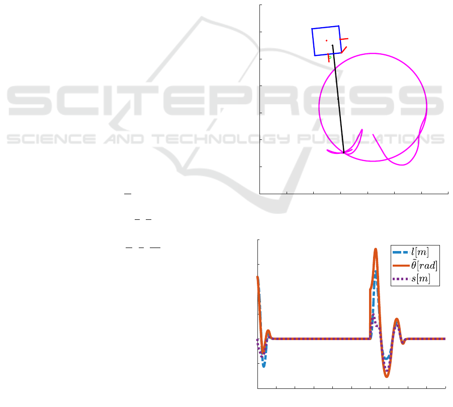
In the Fig 2 we present overall process of following a
path and in the Fig. 4 we can see errors in orthogonal
space. The errors are converging to 0, thus the path is
followed. In 600 second we change the desired path
0 0.5 1 1.5 2 2.5 3 3.5
x [m]
-1
-0.5
0
0.5
1
1.5
2
2.5
y [m]
Figure 3: Full trajectory of the satellite.
0 100 200 300 400 500 600 700 800 900 1000
time [s]
-0.4
-0.2
0
0.2
0.4
0.6
0.8
errors
Figure 4: Errors in orthogonal parametrization space.
ICINCO 2018 - 15th International Conference on Informatics in Control, Automation and Robotics
256

to a fixed point with orientation where the errors also
converge to zero and the satellite in not moving any
more.
7 CONCLUSIONS
The orthogonal path parametrization was presented
for a space object – a flat satellite with 2 DoF pla-
nar manipulator arm. This approach was utilized for
a certain scenario where a flat satellite was used to
chase a object, debris or an other satellite, and du-
ring this manoeuvre the manipulator arm is fixed in
a certain position. The orthogonal path parametriza-
tion was used to track a path parametrized with time
where end effector of the manipulator was moving on
the orbit around the chased object. The most impor-
tant advantage of this approach is very scatter amount
of information needed to successfully follow the path.
The presented method only requires the distance to
the object and orientation error between the followed
path and the current orientation of the satellite. These
type of data, in cosmic conditions, can be relatively
easily collected. Presented manoeuvre in simulation
study section shows two phases of the movement. Fir-
stly, the satellite is following the orbit and then in the
second stage it settles in a point on this path with desi-
red orientation. This is good starting point to intercept
the chased object with only the manipulator and wit-
hout the thrusters as presented in our other research
paper. Further research would involve merging those
to stages into a single manoeuvre.
ACKNOWLEDGEMENTS
The works of Wojciech Domski was sup-
ported by National Science Centre grant no.
2015/17/B/ST7/03995. The works of Alicja Mazur
was supported by the Wrocław University of Science
and Technology statutory grant 0401/0142/17.
REFERENCES
C. M. Allen, A., Langley, C., Mukherji, R., B. Taylor, A.,
Umasuthan, M., and D. Barfoot, T. (2008). Rendez-
vous lidar sensor system for terminal rendezvous, cap-
ture, and berthing to the international space station.
Diaz, J. and Abderrahim, M. (2006). Visual inspection
system for autonomous robotic on-orbit satellite ser-
vicing. in: Proc. 9th ESA Symposium on Advanced
Space Technologies in Robotics and Automation (AS-
TRA 2006).
Do, K. D. and Pan, J. (2003). Robust path following of un-
deractuated ships using Serret-Frenet frame. In Pro-
ceedings of the 2003 American Control Conference,
2003., volume 3, pages 2000–2005 vol.3.
Fradkov, A., Miroshnik, I., and Nikiforov, V. (1999). Nonli-
near and Adaptive Control of Complex Systems. Klu-
wer Academic Publishers, Dordrecht.
Kanazaki, M., Yamada, Y., and Nakamiya, M. (2017). Tra-
jectory optimization of a satellite for multiple active
space debris removal based on a method for the tra-
veling serviceman problem. In 2017 21st Asia Pacific
Symposium on Intelligent and Evolutionary Systems
(IES), pages 61–66.
Li, X., Yao, Y., Yang, B., and Wang, L. (2016). Guidance
strategy design for space debris removal using fracti-
onated spacecraft. In 2016 IEEE Chinese Guidance,
Navigation and Control Conference (CGNCC), pages
264–270.
Mazur, A. (2004). Hybrid adaptive control laws sol-
ving a path following problem for nonholonomic mo-
bile manipulators. International Journal of Control,
77(15):1297–1306.
Rybus, T. and Seweryn, K. (2015). Application of rapidly-
exploring random trees (rrt) algorithm for trajectory
planning of free-floating space manipulator. In 2015
10th International Workshop on Robot Motion and
Control (RoMoCo), pages 91–96.
Siciliano, B. and Khatib, O. (2007). Springer Handbook of
Robotics. Springer-Verlag New York, Inc.
Path Tracking with Orthogonal Parametrization for a Satellite with Partial State Information
257