
Monte Carlo Simulation of Non-stationary Air Temperature
Time-Series
Nina Kargapolova
1,2
1
Laboratory of Stochastic Problems, Institute of Computational Mathematics and Mathematical Geophysics,
Pr. Ak. Lavrent’eva 6, Novosibirsk, Russia
2
Department of Mathematics and Mechanics, Novosibirsk State University, Pirogov St. 2, Novosibirsk, Russia
Keywords: Stochastic Simulation, Non-stationary Random Process, Periodically Correlated Process, Air Temperature,
Temperature Extremes, Model Validation.
Abstract: Two numerical stochastic models of air temperature time-series are considered in this paper. The first model
is constructed under the assumption that time-series are nonstationary. In the second model air temperature
time-series are considered as a periodically correlated random processes. Data from real observations on
weather stations was used for estimation of models’ parameters. On the basis of simulated trajectories, some
statistical properties of rare meteorological events, like sharp temperature drops or long-term temperature
decreases in summer, are studied.
1 INTRODUCTION
The study of statistical properties of atmospheric
processes involving adverse weather conditions (for
example, long-term heavy precipitation, dry hot
wind, unfavourable combination of low temperature
and high relative humidity, etc.) is of great scientific
and practical importance. Results of this study are
crucial for solution of some problems in
agroclimatology, planning of heating and
conditioning systems and in many other applied
areas (see, for example, Pall et al., 2013; Araya and
Kisekka, 2017; Khomutskiy, 2017). Unfortunately,
there are extremely few real observation data for
obtaining stable statistical characteristics of rare /
extreme weather events. Moreover, the behaviour of
their characteristics is influenced by climatic
changes, and hence it is not always possible to
obtain reliable estimates only from observation data.
In this regard, in recent decades a lot of scientific
groups all over the world work at development of
so-called "stochastic weather generators" (or short
"weather generators"). At its core, " weather
generators" are software packages that allow
numerically simulate long sequences of random
numbers having statistical properties, repeating the
basic properties of real meteorological series. Using
the Monte Carlo method, both the properties of
specific meteorological processes and their
complexes are studied (see, for example, Kleiber et
al., 2013; Ailloit et al., 2015; Semenov et al., 1998,
Kargapolova, 2017). Depending on the problem
being solved, time-series of meteorological elements
of different time scales are simulated (with hours,
days, decades, etc. as a time-step). The type of
simulated random processes (stationary or non-
stationary, Gaussian or non-Gaussian, etc.) is
determined by the properties of real meteorological
processes and by the selected time step.
In this paper two numerical stochastic models of
air temperature non-Gaussian time-series are
considered. The first model is constructed under the
assumption that time-series are nonstationary. In the
second model air temperature time-series are
considered as a periodically correlated random
process. Both models let to simulate air temperature
time-series with 3 h. time-step, taking into account
daily oscillation of a real process. Parameters of both
models were estimated on the basis of data from
long-term real observations. On the basis of
simulated trajectories, some statistical properties of
rare meteorological events, like sharp temperature
drops or long-term temperature decreases in
summer, are studied.
Kargapolova, N.
Monte Carlo Simulation of Non-stationary Air Temperature Time-Series.
DOI: 10.5220/0006833403230329
In Proceedings of 8th International Conference on Simulation and Modeling Methodologies, Technologies and Applications (SIMULTECH 2018), pages 323-329
ISBN: 978-989-758-323-0
Copyright © 2018 by SCITEPRESS – Science and Technology Publications, Lda. All rights reserved
323

2 REAL DATA
In this paper a problem connected with the study of
some statistical characteristics of rare and extreme
behavior of air temperature is considered. In order to
solve this problem, one has to construct a numerical
stochastic model of the air temperature time-series
based on real data collected at weather stations. To
define models’ parameters data collected 8 times per
day (i.e. every 3 hours) during 23 years from 1993 to
2015 were used. For the sake of convenience,
month-long time-series of air temperature that start
on the first of a month are considered. The most
noticeable feature of the temperature series at such
time interval is the diurnal variation, defined by the
day/night alternation. As an illustration, on the Fig. 1
temperature in Sochi (Russia) in December 1993 and
2015 is presented. All models, considered in this
paper, were tested on a basis of real data from 12
weather stations situated in different climatic zones
(for example, weather stations in Sochi (subtropical
zone), Ekaterinburg (temperate continental zone),
Tomsk (sharply continental zone), Prigranichniy
(polar zone), etc.). Although all examples in the
article are given only for Sochi and Tomsk, all
conclusions are valid for all considered weather
stations.
Figure 1: Air temperature. Sochi. December, 1-11.
3 PERIODICALLY
CORRELATED MODEL
Recall that a random process
Xt
is a periodically
correlated process with a period
T if its
mathematical expectation, variance and correlation
function are periodic functions (Gladyshev, 1961;
Dragan et al., 1987):
12 1 2
,,
,,.
EX t EX t T DX t DX t T
corr X t X t corr X t T X t T
The idea of simulation of Gaussian sequences
satisfying these conditions belongs to V.A. Rozhkov
and was first realized in the form of a first-order
autoregression vector model (Bokov et al., 1995).
Later, other approaches to simulation of random
processes with such properties were developed (see,
for example, Hurd and Miamee, 2007; Kargapolova
and Ogorodnikov, 2012; Ogorodnikov et al., 2010;
Sereseva and Medvyatskaya, 2017).
The idea to consider air temperature time-series
as periodically correlated processes with a period
equal to 24 hours was suggested in (Derenok and
Ogorodnikov, 2008). However, due to ill-considered
choice of approximation of sample one-dimensional
distributions, the proposed model gave acceptable
results in the study of extreme temperature behavior
only for weather stations located in a temperate
climatic zone. In this paper a modification of a
model, suggested in (Derenok and Ogorodnikov,
2008), is presented. This modification gives good
results for all considered climatic zones.
Let’s consider time-series
12 8
,,,
d
TTT T
of
air temperature as a periodically correlated discrete-
time random process with a period
8T
, where
i
T
is air temperature at a measurement number
i
(“at a
time moment
i
” ),
28,30,31d
is a number of
days in a month.
First input parameter of a stochastic model is
one-dimensional distribution of each component
i
T
.
To construct a stochastic model, the use of sample
one-dimensional distributions is not advisable, since
the sample distributions don’t have any tails, and
therefore do not allow to estimate the probability of
occurrence of extreme values of a meteorological
element. In this connection, it is necessary to
approximate the sample distributions by some
analytic densities, which, on the one hand, do not
greatly alter the form of the distribution and its
moments, and on the other, possess tails. In
(Derenok and Ogorodnikov, 2008) a Gaussian
density was used for such approximation. Analysis
of real data shows that at some weather stations
sample distribution of air temperature is bimodal,
and it can’t be approximated well with a Gaussian
distribution. To define the best approximation (in
sense of the Pearson’s criterion and closeness of
approximating distributions moments to empirical
ones) several types of approximating densities and
different methods of densities parameters estimation
were compared. Numerical experiments show that
mixtures
SIMULTECH 2018 - 8th International Conference on Simulation and Modeling Methodologies, Technologies and Applications
324
2
1
2
1
1
2
2
2
2
2
1
exp
2
2
1
1exp ,
2
2
k
kk
k
k
k
k
k
k
xa
gx
b
b
xa
b
b
01,1,8.
k
k
of two Gaussian distributions approximate closely
sample histograms of air temperature for all
measurements
1, 8k
(and, therefore, for all
moments of time
1, 2, , 8id
) at all considered
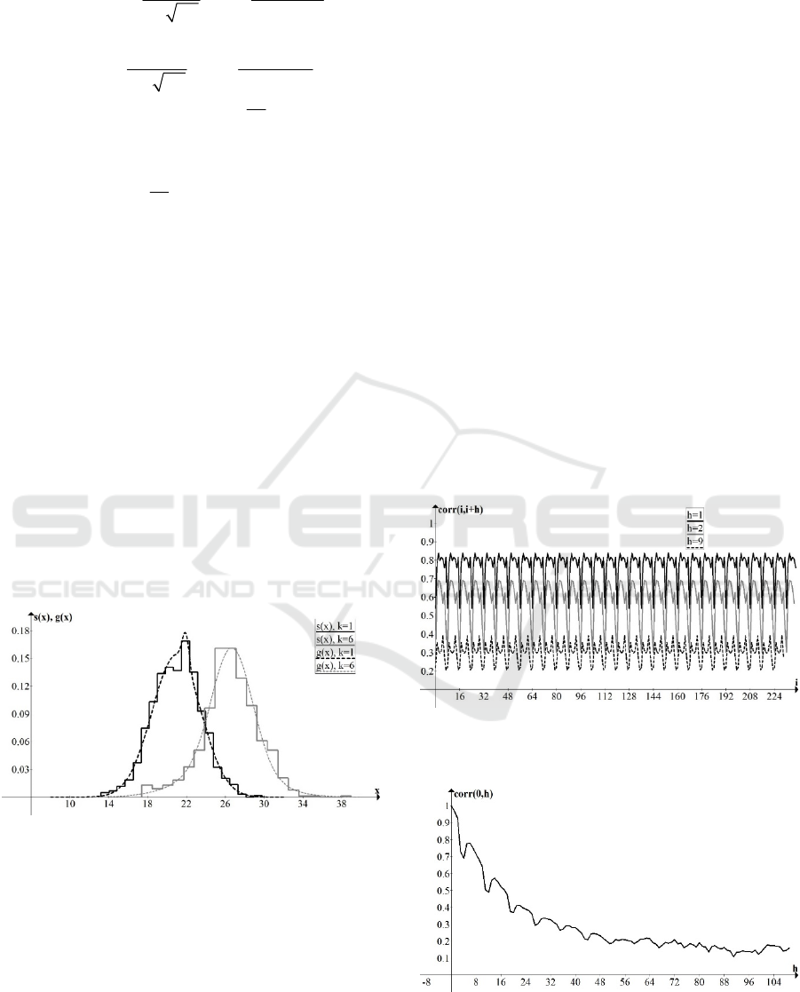
weather stations. Fig. 2 shows examples of air
temperature sample histograms
,
o
k
s
xxC
and
corresponding approximating densities. Parameters
22
11 2 2
,,,,
kk k k k
abab
were chosen using an
algorithm, proposed in (Marchenko and Minakova,
1980). This algorithm let to choose such parameters
of a mixture
k
g
x
that mathematical expectation,
variance and skewness of a random variable with a
density
k
g
x
are equal to corresponding sample
characteristics and function
k
g
x
minimizes the
Pearson’s functional, that describes difference
between
k
s
x
and
k
g
x
. For each
k
sample
mathematical expectation, variance and skewness
were estimated on a basis of
23d
-element sample.
Figure 2: Sample and approximation distribution densities
of air temperature. Sochi, July.
Another input parameter of a model is
correlation matrix of the weather process. In this
paper a sample correlation matrix
R is used to
describe correlation structure of air temperature
time-series (approximation of the sample correlation
function of the process with some analytic
parametric function is a work in progress). It should
be noted, that the matrix
11 18
81 88
,,
,,
1,1 1, 8
,
8,1 8,8
d
ddd
corr T T corr T T
R
corr T T corr T T
corr corr d
corr d corr d d
estimated under assumption that the process T
is
periodically correlated, is a block-Toeplitz matrix.
Analysis of real data shows that for all
meteorological stations and months considered, the
amplitudes of diurnal oscillations of the
corresponding autocorrelation functions
,corr i i h
of air temperature are significant.
Fig. 3 shows examples of sample correlation
coefficients
,corr i i h
, as functions of time
i
for
a fixed shift
h
(presented in Fig. 3 functions are
periodic because estimations of correlation
coefficients were done under the assumption that the
process
T
is periodically correlated). As a function
of the shift
h
, the correlation coefficients decrease
rapidly, as illustrated in Fig. 4.
Figure 3: Sample correlation coefficients
,corr i i h
of air temperature. Tomsk, June.
Figure 4: Sample correlation coefficients
0,corr h
of
air temperature. Sochi, December.
Monte Carlo Simulation of Non-stationary Air Temperature Time-Series
325

For simulation of
T
with given one-dimensional
distributions
,1,8
k
gxk
and given correlation
matrix
R a method of inverse distribution function
may be used (Piranashvili 1966; Ogorodnikov and
Prigarin, 1996). In the framework of this method,
simulation of
T
comes down to an algorithm with 3
steps:
1.
Calculation of a matrix
R
that is a correlation
matrix of an intermediate standard Gaussian
process
12 8
,,,
d
TTT T
. Element
i, j , , 1,8rijd
of the matrix
R
is a
solution of an equation
11
i, j
i, j,, ,
ij
Fx
cor
F
yxy dxd
r
ry
where
2
2
22
,,
2
21 exp
2
i, j
i, j
i, j
ij1,
xy
xy x y
r
r
r
r
is a distribution density of a bivariate Gaussian
vector with zero mean, variance equal to
1 and
correlation coefficient
i, jr
between components
number
i
and j ,
is a CDF of a standard
normal distribution,
,
ij
F
F
are CDFs corresponding
to densities
,
ij
g
xgx.
2.
Simulation of a standard Gaussian sequence T
with correlation matrix
R
.
3.
Transformation of T
into T
:
1
,1,8
ii i
TF T i d
.
If matrix
R
, obtained in the first step, is not
positively defined, it must be regularized. Several
methods of regularization are described in
(Ogorodnikov and Prigarin, 1996). In this paper a
method of regularization based on substitution of
negative eigenvalues of the matrix
R
with small
positive numbers was used. Simulation of a standard
Gaussian sequence
T
with correlation matrix
R
in
the second step could be done using Cholesky or
spectral decomposition of the matrix
R
. However,
due to a special structure of the matrix
,R
there are
methods to reduce time required for simulation of
T
. As it was mentioned above, matrix R is a
block-Toeplitz matrix. Therefore, matrix
R
is also
block-Toeplitz. This means that the sequence
T
may be interpreted as a vector stationary sequence,
that could be simulated with efficient algorithms
presented in (Ogorodnikov, 1990; Robinson, 1983).
In this paper an algorithm of Levinson was used. It
should be noted that, due to the block-Toeplitz
structure of the matrix
R
, on the first step of the
simulation algorithm, it is enough to solve only
88d
equations for
i, j , 1, 8, 1, 8rijd
.
4 NONSTATIONARY MODEL
It is possible to consider air temperature time-series
as a non-stationary sequence without any periodic
characteristics. At first thought, this assumption
looks especially plausible for off-season months,
when difference between average daily temperature
in the beginning and in the end of a month is
essential. Fig. 5 shows an example of fluctuation of
average temperature in such month.
Figure 5: Average daily air temperature. Tomsk,
November.
For simulation of a non-stationary sequence
12 8
,S , ,
d
SS S
of air temperature it is
necessary to define
8d
distribution densities
(instead of
8
densities in the periodically correlated
model). As in the described above model, in the non-
stationary model for approximation of sample
histograms mixtures of Gaussian distributions are
used. It should be noted that in this case size of a
sample used for histogramming and estimation of
sample moments is equal to
23
. Since sample is so
small, the statistical uncertainty of distribution
parameters estimation is relatively great. To
decrease this uncertainty, a moving average
procedure with a five-day averaging window was
SIMULTECH 2018 - 8th International Conference on Simulation and Modeling Methodologies, Technologies and Applications
326

used for distribution parameters and correlation
coefficients estimation.
Sample correlation matrix
i, jCc
of a
non-stationary sequence
S
, used as a second input
parameter of a model, doesn’t have any specific
features. It means that in the framework of inverse
distribution function method it is necessary to solve
88dd
equations to define a correlation matrix
i, jCc
of an auxiliary standard Gaussian
process
'S
. In this paper simulation of
'S
with the
correlation matrix
C
was done using Cholesky
decomposition of the matrix
C
.
5 NUMERICAL EXPERIMENTS
It is obvious, that any stochastic model must be
verified before one starts to use simulated
trajectories to study properties of a simulated
process. For a model verification, it is necessary to
compare simulated and real data based estimations
of such characteristics, which, on the one hand, are
reliably estimated by real data, and on the other hand
are not input parameters of the model. Here are
several examples of such characteristics.
Tab. 1 shows the probabilities of the event “air
temperature is below a given level
o
lC
during at
least 3 hours (equivalently – during at least 2
consequent measurements)”. For models
verification, levels
l
close to the mean values of
temperature were chosen. Since both models
accurately reproduce this characteristic, simulated
trajectories were used to estimate the probabilities of
the specified event for extreme low levels (
38, 40
o
lC
) for which an estimate from a small
sample of real data yields a zero result, although the
event is possible. Here and below
5
10
simulated
trajectories were used for estimations. To denote
estimations based on real data, an abbreviation RD is
used, and for estimations based on the periodically
correlated model and on the nonstationary one
abbreviations PCM and NSM are used respectively.
Another characteristic that was used both for
models verification and study of air temperature
time-series properties was a “probability of a rapid
change of air temperature”. As a rapid change of air
temperature, a change for more than
o
C
in less
than 24 hours was considered. Tab. 2 shows
corresponding estimations. Rapid temperature
changes (both temperature drops and rises) are
unpleasant weather events, that negatively influence
on a human well-being and on open-ground planted
crop species. This characteristic is reproduced well
by both models for all considered weather stations.
Table 1: Probabilities of the event "air temperature is
below a given level
o
lC
during at least 3 hours". Tomsk,
December.
o
lC
RD PCM NSM
-10 0.63 0.61 0.62
-14 0.46 0.44 0.42
-16 0.37 0.38 0.40
-18 0.31 0.20 0.31
-32 0.04 0.03 0.04
-38 0.00 0.01 0.01
-40 0.00 0.01 0.01
Table 2: Probabilities of the air temperature rapid change.
Tomsk, March.
o
C
RD PCM NSM
5 0.85 0.84 0.86
9 0.52 0.54 0.51
13 0.23 0.23 0.22
17 0.06 0.05 0.07
21 0.01 0.02 0.02
25 0.00 0.01 0.01
One more characteristic that was studied on a
basis of real and simulated data was “average
number of days in a month with a minimum daily
temperature above given level
o
lC
”. Tab. 3 shows
corresponding estimations. That last column of the
Tab. 3 contains estimations of the characteristic
under consideration, obtained with simulated
trajectories of a well-known model WGEN (see, for
example, Richardson, 1981; Richardson and Wright,
1984; Semenov et al., 1998). WGEN is a stochastic
model of a weather complex “daily precipitation,
daily maximum and minimum temperature, solar
radiation”. All three models (PCM, NSM and
WGEN) give comparable results. It's worth noting
that for extreme high levels
26,28
o
lC
there is a
big difference between estimations on real and
simulated data. The most probable explanation of
this fact is that size of a real data sample is too small
for reliable estimation of rare (but physically
possible) weather events.
The last characteristic presented in this paper is
“average daily temperature in a day number
i
”.
Estimations of these probabilities for two different
months (first of which is an in-season month and
second is an off-season) are shown in Tab. 4 and
Monte Carlo Simulation of Non-stationary Air Temperature Time-Series
327

Tab.5. It’s easy to see, that NSM accurately
reproduces this characteristic both for in-season and
off-season months, while PCM gives plausible
results only for the in-season month.
Table 3: Average number of days in a month with a
minimum daily temperature above given level
o
lC
.
Sochi, July.
o
lC
RD PCM NSM WGEN
14 30.78 30.81 30.76 30.80
16 29.83 29.63 29.64 29.60
18 25.70 25.31 25.98 25.30
20 16.74 16.70 16.79 16.70
22 7.09 6.96 7.03 7.07
24 1.70 1.63 1.62 1.60
26 0.04 0.21 0.20 0.19
28 0.00 0.11 0.11 0.10
Table 4: Average daily temperature in a day number i .
Sochi, January.
i
RD PCM NSM
1 7.41 7.42 7.39
11 6.17 6.16 6.19
21 5.69 5.66 5.63
31 5.84 5.83 5.81
Table 5: Average daily temperature in a day number i .
Sochi, May.
i
RD PCM NSM
1 13.87 16.01 13.96
11 15.99 16.06 15.83
21 18.47 15.99 18.01
31 19.45 16.04 19.52
6 CONCLUSIONS
Results of numerical experiments show that, in
general, both considered models reproduce quite
well the properties of a real air temperature time-
series in an in-season month and can be used for
study of the properties of extreme / rare
meteorological events. But, since simulation of a
periodically correlation sequence
'T
as a vector
stationary sequence requires less time than
simulation of a non-stationary sequence
'S
, usage
of the first model is preferable. For off-season
months the periodically correlated model does not
always give satisfactory results, so it is better to use
the non-stationary model.
In future, the both models will be expanded –
instead of air temperature time-series, three-
component weather complexes “air temperature,
relative humidity, atmospheric pressure” and “air
temperature, relative humidity, wind speed
modulus” will be simulated as joint time-series.
Simulation of first weather complex is of interest,
because on a basis of simulated trajectories it is
possible to study the properties of humid air
enthalpy time-series. Simulated trajectories of the
second complex could be used as input data for
models of forest / grassland fires spread.
Both models also could be easily transformed
into conditional models that may be used for
probabilistic forecasting of air temperature. Quality
of such forecasts will be studied later.
ACKNOWLEDGEMENTS
Author is deeply indebted to Prof. V. Ogorodnikov
for his help and fruitful discussions.
This work was partly financially supported by
the Russian Foundation for Basis Research (grant
No 18-01-00149-a) and the President of the Russian
Federation (grant No MK-659.2017.1).
REFERENCES
Ailliot, P., Allard, D., Monbet, V., Naveau, P., 2015.
Stochastic weather generators: an overview of weather
type models. In Journal de la Société Française de
Statistique, Vol. 156, No 1. P. 101-113.
Araya, A., Kisekka, I., 2017. Evaluating the impact of
future climate change on irrigated maize production in
Kansas. In Climate Risk Management, Vol. 17. P. 139-
154.
Bokov, V.N., Lopatukhin, L.I., Mikulinskaya, S.M.,
Rozhkov, V.A., Rumyantseva, S.A., 1995. Inter-year
variability of sea heaving. In Prob. of Study and Math.
Modelling of Wind Agitation, Gidrometeoizdat,
St.Petersburg. P. 446-454. (in Russian)
Derenok, K.V., Ogorodnikov, V.A., 2008. Numerical
simulation of significant long-term decreases in air
temperature. In Russ. J. Num. Anal. Math. Modelling,
Vol. 23, No 3. P. 223-277.
Dragan, Ya.P., Rozhkov, V.A., Yavorskii, I.N., 1987.
Methods of probabilistic analysis of rhythmic of
oceanology processes, Gidrometeoizdat, Leningrad.
(in Russian)
Gladyshev, E.G., 1961. Periodically correlated random
sequences. In Dokl. Akad. Nauk SSSR, Vol. 137, No 5.
P. 1026-1029.
Hurd, H.L., Miamee, A., 2007. Periodically Correlated
Random Sequences: Spectral Theory and Practice,
John Wiley & Sons, Inc.
Kargapolova, N. A., 2017. Stochastic “weather
generators”. Introduction to stochastic simulation of
meteorological processes, PPC NSU, Novosibirsk.
SIMULTECH 2018 - 8th International Conference on Simulation and Modeling Methodologies, Technologies and Applications
328

Kargapolova, N.A., Ogorodnikov, V.A., 2012.
Inhomogeneous Markov chains with periodic matrices
of transition probabilities and their application to
simulation of meteorological processes. In Russ. J.
Num. Anal. Math. Modelling, Vol. 27, No 3. P. 213-
228.
Khomutskiy Ju., 2017, Usage of observed temperature
data for designing of air conditioning and ventilation
systems. In World of Climate, Vol. 101. P. 156-161.
(in Russian)
Kleiber, W., Katz, R.W., Rajagopalan, B., 2013. Daily
minimum and maximum temperature simulation over
complex terrain. In Annals of Applied Statistics, No 7.
P. 588-612.
Marchenko, A.S., Minakova, L.A., 1980. Probabilistic
model of air temperature time-series. In Meteorology
and Hydrology, No. 9. P. 39-47. (in Russian)
Ogorodnikov, V.A., 1990. Statistical simulation of
discrete random processes and fields. In Sov. J. Num.
Anal. Math. Modelling, Vol. 5, No 6. P. 489-509.
Ogorodnikov, V.A., Prigarin S.M., 1996. Numerical
Modelling of Random Processes and Fields:
Algorithms and Applications, VSP, Utrecht.
Ogorodnikov, V.A., Derenok, K.V., Tolstykh, U.I., 2010.
Special numerical models of discrete random series. In
Russ. J. Num. Anal. Math. Modelling, Vol. 25, No 4.
P. 359-373.
Pall, R.K., Sehgal, V.K., et al., 2013. Application of
Seasonal Temperature and Rainfall Forecast for Wheat
Yield Prediction for Palampur, Himachal Pradesh. In
Int. J. of Agriculture and Food Sc. Tech., Vol. 4, No 5.
P. 453-460.
Piranashvili, Z.A., 1966. Some problems of statistical
probabilistic modelling of random processes. In Probl.
of Operations Res., Tbilisi, P. 53-91. (in Russian)
Richardson, C.W., 1981. Stochastic simulation of daily
precipitation, temperature and solar radiation. In Water
Resour. Res., Vol. 17, No 1. P. 182–190.
Richardson, C.W., Wright, D.A., 1984. WGEN: A Model
for Generating Daily Weather Variables, U. S.
Department of Agriculture, Agricultural Research
Service.
Robinson, E.A. 1983. Multichannel time series analysis
and digital computer program, Goose Pond Press,
Houston.
Semenov, M.A., Brooks, R.J., Barrow, E.M., Richardson,
C.W., 1998. Comparison of the WGEN and LARS-
WG stochastic weather generators for diverse
climates. In Climate Res., Vol. 10. P. 95-107.
Sereseva, O.V., Medvyatskaya, A.M., 2017. Numerical
stochastic model of the joint periodically correlated
process of air temperature and relative humidity. In
Proceedings of the International Workshop «Applied
Methods of Statistical Analysis. Nonparametric
Methods in Cybernetics and System Analysis», P. 285-
291.
Monte Carlo Simulation of Non-stationary Air Temperature Time-Series
329
