
Using Machine Learning for Recommending Service Demand Estimation
Approaches - Position Paper
Johannes Grohmann, Nikolas Herbst, Simon Spinner and Samuel Kounev
Universit
¨
at W
¨
urzburg, Am Hubland, 97074 W
¨
urzburg, Germany
Keywords:
Service Demand Estimation, Machine Learning, Approach Selection, Service Modeling.
Abstract:
Service demands are key parameters in service and performance modeling. Hence, a variety of different
approaches to service demand estimation exist in the literature. However, given a specific scenario, it is not
trivial to select the currently best approach, since deep expertise in statistical estimation techniques is required
and the requirements and characteristics of the application scenario might change over time (e.g., by varying
load patterns). To tackle this problem, we propose the use of machine learning techniques to automatically
recommend the best suitable approach for the target scenario. The approach works in an online fashion and
can incorporate new measurement data and changing characteristics on-the-fly. Preliminary results show that
executing only the recommended estimation approach achieves 99.6% accuracy compared to executing all
approaches available, while speeding up the estimation time by 57%.
1 INTRODUCTION
Optimizing performance of applications in modern
day cloud environments usually aims at minimizing
the allocated resources while still complying with cer-
tain Service Level Objectives (SLOs). Service de-
mands (also known as resource demands) can help to
reach that goal. A service demand is the average time
a unit of work (e.g., request or transaction) spends
obtaining service from a resource (e.g., CPU or hard
disk) in a system over all visits excluding any wait-
ing times (Menasc
´
e et al., 2004). Requests can be
grouped into different workload classes with similar
service demands.
Timely and precise service demands can be uti-
lized by other tools optimizing the resource alloca-
tion in a cloud environment, including proactive auto-
scaling mechanisms used for elastic resource provi-
sioning (Bauer et al., 2017), stochastic performance
models such as Queueing Networks (QN) (Bolch
et al., 1998), Queueing Petri Nets (QPN) (Bause,
1993), or architecture-level performance models such
as the Descartes Modeling Language (DML) (Kounev
et al., 2016).
Over the years, a number of approaches to Service
Demand Estimation (SDE) have been proposed using
different statistical estimation techniques (e.g., linear
regression (Rolia and Vetland, 1995; Brosig et al.,
2009) or Kalman filters (Wang et al., 2012; Zheng
et al., 2008) and based on different laws from queue-
ing theory. When selecting an appropriate approach
for a given scenario, a user has to consider different
characteristics of the estimation approach, such as the
expected input parameters, its accuracy and its robust-
ness to measurement anomalies. Depending on the
constraints of the application context, only a subset of
the estimation approaches may be applicable (Spinner
et al., 2015).
Naturally, one wants to select the suitable (e.g.,
best, fastest or a combination of both) approach for
a given scenario. This is especially challenging in
online settings, where the load patterns, the system
structure and even the application architecture and
therefore the characteristics of the service demand es-
timates may not be known in advance and may change
frequently. This also eliminates the possibility for an
expert guess, since this guess has to be repeated in
certain periods.
We therefore propose the use of machine learn-
ing techniques to select the suitable approach in this
context. Given a representative data set, we can train
different Machine Learning Algorithms (MLAs) with
the performance and the time-to-result of different
estimators. During live production, the pre-trained
MLA can be used to predict the most suitable ap-
proach (subject to certain criteria) in the current sce-
nario.
This work aims at providing a proof-of-concept.
Our contributions in this paper are:
1. We list the features that proved to be useful for the
Grohmann, J., Herbst, N., Spinner, S. and Kounev, S.
Using Machine Learning for Recommending Service Demand Estimation Approaches - Position Paper.
DOI: 10.5220/0006761104730480
In Proceedings of the 8th International Conference on Cloud Computing and Services Science (CLOSER 2018), pages 473-480
ISBN: 978-989-758-295-0
Copyright
c
2019 by SCITEPRESS – Science and Technology Publications, Lda. All rights reserved
473

recommendation of SDE approaches.
2. We evaluate three MLAs (Decision Tree (DT),
Support Vector Machine (SVM), Neural Network
(NN)) with regard to their recommendation capa-
bilities.
3. We show the benefit (time saving) and the draw-
back (accuracy loss) of recommendation for SDE.
The remainder of the paper is structured as fol-
lows. We list the related work and the approaches
considered in this paper in Section 2. Section 3 ex-
plains our approach in more detail. We present pre-
liminary results in the offline scenario in Section 4
and give a small outlook into our future planned work
in Section 5. We summarize our statements in Sec-
tion 6
2 RELATED WORK
Next to Filling-the-Gap (Wang et al., 2015), the only
publicly available tool providing different ready-to-
use approaches to service demand estimation is the
Library for Resource Demand Estimation (LibReDE)
by (Spinner et al., 2014).
1
LibReDE currently sup-
ports implementations of the following eight estima-
tion approaches:
• Service Demand Law (Brosig et al., 2009)
• Approximation with response times (Brosig et al.,
2009)
• Least Squares (LSQ) regression using queue-
lengths and response times (Kraft et al., 2009)
• LSQ regression using utilization law (Rolia and
Vetland, 1995)
• Kalman Filter (KF) using utilization law (Wang
et al., 2012; Wang et al., 2011)
• KF using response times and utilization (Zheng
et al., 2008; Kumar et al., 2009)
• Recursive optimization using response
times (Menasc
´
e, 2008)
• Recursive optimization using response times and
utilization (Liu et al., 2006)
Further approaches for SDE can be found in this
survey (Spinner et al., 2015). For lack of space,
we can not go into detail about the used approaches
and refer to the original papers or the LibReDE user
guide (Spinner et al., 2014).
1
LibReDE: Available for download at
http://descartes.tools/librede.
Note that there are different methodologies (sim-
ple approximation, LSQ regession, KF and mathe-
matical optimization) involved. This leads to a wide
diversity in terms of run-time and estimation quality
in different scenarios. This was established by com-
paring the performance of the estimators in different
scenarios, e.g. by varying resource utilization or the
number of workload classes (Spinner et al., 2015).
Linear Regression (LR) techniques were quite
thoroughly investigated in literature, including the im-
pact of different factors and limitations of LR in ser-
vice demand estimation (Rolia and Vetland, 1995;
Rolia and Vetland, 1998; Pacifici et al., 2008; Casale
et al., 2008; Casale et al., 2007; Stewart et al., 2007).
Other works compare LSQ regression with Maximum
Likelihood Estimation (MLE) (Kraft et al., 2009)
or Independent Component Analysis (ICA) (Sharma
et al., 2008). The performance of KFs for service
demand estimation is investigated by (Zheng et al.,
2005; Zheng et al., 2008; Kumar et al., 2009).
In our prior work (Grohmann et al., 2017), we
used generic optimization methods to optimize the
parameter settings of the aforementioned approaches
for the given target scenario. Our work in this paper
can be seen as orthogonal and complementary to this,
since the recommendation uses the approaches as-is.
3 APPROACH SELECTION
METHODOLOGY
This section describes our idea for using MLAs for
the selection of SDE approaches at run-time.
In order to be able to predict the best SDE ap-
proach, we need to create a model on a labeled train-
ing set. This training set consists of time series of sys-
tem metrics. We use these traces to estimate service
demands using the different approaches and validate
the results via cross-validation.
After running all estimation approaches, we can
extract several features about each trace. These fea-
tures can be used to characterize and categorize the
traces. The MLAs are fed with the extracted features,
as well as with the approach that worked best on the
respective trace. After the training is completed, the
defined features can also be extracted for new and
so far unseen traces. With these, the trained MLAs
model can predict the approach that should work best
on the respective trace.
We define the machine learning problem as a
classification problem. We have a labeled data set
{(x
1
,y
1
),...,(x
n
,y
n
)} assigning each feature vector
X
i
a label y
i
. The label represents the best SDE ap-
proach in the given situation (based on the minimum
CLOSER 2018 - 8th International Conference on Cloud Computing and Services Science
474

cross-validation error). Given that we consider 8 dif-
ferent SDE approaches in our experiments, we dis-
tinguish between 8 different classes. The vectors x
i
contain one real number for each feature, i.e. x
i
∈ R
k
,
where k is the number of features.
After the training is complete, the obtained model
can be used to select the best suitable SDE approach
at run-time. The training set can consist of an offline
data set, which was collected beforehand or it can
be extended dynamically in an online fashion. If
the training set is augmented during live production,
training processes can be repeated arbitrarily often al-
though this might take up some time depending on the
size of the training set and the complexity of the used
features.
The intervals of when a current trace should be
archived to the training set, when the model should
be retrained and when the selection of the current ap-
proach should be executed are variable. This opens
room for configuration and experimentation.
Note that due to the use of cross-validation to rank
the different SDE approaches, no manual labeling or
interaction is required during the creation of the train-
ing set. (Since all approaches can be tried and the
one with the highest score is chosen.) Hence, large
amounts of data from different computing clusters of
the cloud can be used as training set very easily. Also,
the model is able to increase it’s training set continu-
ously during production and therefore learn from its
own mistakes.
We list the features, we consider in Section 3.1 and
describe different MLAs we use for recommendation
in Section 3.2
3.1 Features
This section contains the list of features we extract to
train the algorithms. Features are certain characteris-
tics of the input traces used by the system to extract
knowledge about the traces.
The MLAs are heavily dependent on those fea-
tures and a careful selection as well as the right
amount is crucial for a satisfactory outcome. Since
the MLAs try to distinguish between different classes
of traces, too many features can actually be harm-
ful. However, it is generally a good idea to collect
as many features as possible at first and then decide
later, which are the most informative. In some cases,
this decision can even be left to the MLA itself.
In the following, trace refers to one training ex-
ample of our data set. A trace usually consists a time
series of the CPU-utilization of each resource, the re-
sponse time and the arrival rate of each request of
the respective workload classes for feature generation.
The CPU-utilization measures the average utilization
of the CPU for a certain interval, the response time
contains the response time of each request and the ar-
rival rate holds the number of incoming requests for
a certain interval. These traces are given to the SDE
approaches for their estimations. For each trace, we
want to create a feature representation y
i
(see previous
section) that captures the characteristics of this trace.
Furthermore, we have some general meta-
information about the traces holding the number of
resources (e.g. number of CPUs and/or CPU cores)
and the number of different workload classes (i.e. dif-
ferent request types/methods). The number of work-
load classes already has a direct impact on the perfor-
mance of the estimators as shown by (Spinner et al.,
2015). Therefore, we include this meta-information
as features.
Additionally, we extract statistical information
about the traces as features. (Spinner et al., 2015)
show for example that the utilization has a significant
impact on some of the estimators. It is therefore use-
ful to include information about the average utiliza-
tion of the available resources as well as the minimum
and the maximum utilization.
However, it does not seem useful to average this
information over all resources. Especially the differ-
ent workload classes are characteristic for having dif-
ferent values. We therefore define a set of statistical
features, extract those for each resource (utilization
features) and workload class (arrival rate and response
time features) and concatenate them to one feature
vector y
i
.
This limits the number of maximum resources and
workload classes to process. In order to be able to
concatenate all features to one vector, we need to de-
fine a maximum number of resources and workload
classes used for training. If a trace has less statisti-
cal features, the remaining values can be filled with
zeros.
The extracted statistical features for the set of data
points d = (d
1
,...,d
n
) are:
The number of samples n per trace.
The arithmetic average: d =
1
n
∑
n
i=1
d
i
.
The geometric average:
ˆ
d = (
∏
n
i=1
d
i
)
1
n
.
The standard deviation: σ =
q
1
n
∑
n
i=1
(d
i
− d)
2
.
The quadratic average or Root Mean Square (RMS):
x
rms
=
q
1
n
d
2
1
+ d
2
2
+ ··· + d
2
n
.
The minimum value in d.
The maximum value in d.
Using Machine Learning for Recommending Service Demand Estimation Approaches - Position Paper
475

The kurtosis of d, a measure for the tailed-
ness of the graph of d, see (Westfall, 2014):
k =
1
n
∑
n
i=1
(d
i
−d)
4
1
n
∑
n
i=1
(d
i
−d)
2
2
− 3.
The skewness of d, a measure for asymme-
try. See (Joanes and Gill, 1998): s =
1
n
∑
n
i=1
(d
i
−d)
3
h
1
n−1
∑
n
i=1
(d
i
−d)
2
i
3/2
.
The 10
th
percentile. Below this point are 10% of the
total points in d.
The 90
th
percentile. Below this point are 90% of the
total points in d.
Omitted features: Furthermore, it seems useful
to include correlation information about the traces.
However, as the whole idea of the online selection is
to improve the speed of the SDE, the feature calcula-
tion (which is done online as well) has to be reason-
ably fast as well.
We experimented with features regarding the cor-
relations and the covariances between the traces, the
Variance Inflation Factor (VIF) and information about
the statistical distributions. However, those are costly
to calculate and as they did not show any improve-
ments in our experiments, we decided not to include
them in the feature set. Instead, we focus on the fea-
tures mentioned above. For the results of the aug-
mented feature set, see (Grohmann, 2016).
The total number of features is therefore k = 2 +
11 · r + 22 · w, with r being the number of resources
and w being the number of workload classes in the
training set.
3.2 Algorithms
For our proof-of-concept, we limit ourselves to im-
plement three MLAs..
Decision Tree: DTs are a well-known and intuitive
way to cluster information that is quite easy to under-
stand for a human supervisor (Breiman et al., 1984).
For splitting decisions we use the Gini impurity I
G
by (Breiman et al., 1984). It measures how pure a
split is, i.e. the average probability of an an element
of the node to be labeled wrong if it was randomly
classified according to the relative frequencies of the
node. It is calculated with
I
G
( f ) =
J
∑
i=1
f
i
(1 − f
i
), (1)
if J is the number of classes and f
i
the fraction of
classes labeled with label i, i.e. the probability to ran-
domly draw class i for a given element. Note that I
G
reaches its minimum value at zero if all the elements
belong to the same class. The Gini impurity has there-
fore to be minimized, in order to create pure trees.
To avoid over-fitting, we limit the amount of nodes
in the DT to 100.
Support Vector Machines: SVMs have many pa-
rameters and configuration options (Russell and
Norvig, 2009). The correct configuration of them
poses an optimization problem itself. For our experi-
ments we use a Gaussian kernel function
K(x,y) = exp
kx + yk
2
σ
, (2)
with σ = 8 and a soft-margin penalty of 5. We face the
multi-class problem with the one-vs-all strategy. Ac-
cording to a small grid-search, this proved to perform
best on our data set.
Neural Networks: Our implementation of a NN
is a multi-layer sigmoid-perceptron with its nodes
fully connected by acyclic arcs, prohibiting feedback
loops. We decided to use two inner layers (since two
inner layers are enough to represent any kind of func-
tion (Cybenko, 1988)), resulting in a total of four lay-
ers if we add the input and the output layer. We limit
ourselves to 100 neurons excluding the input layer in
order to ensure the fast processing of the recommen-
dation algorithm. Therefore, we kept the number or
neurons (and especially the number of layers) reason-
ably small.
The output layer consists of one node for each
available estimator (currently eight), resulting in 46
fully connected nodes for each of the inner layers.
We use the back-propagation algorithm (Bryson
and Ho, 1969) with five epochs for training. LSQ
serves as error function and the sigmoid function in
equation 3 as activation function for each neuron:
S(t) =
1
1 + e
−t
. (3)
The sigmoid function is a popular choice in the litera-
ture as it offers nice mathematical properties (Russell
and Norvig, 2009).
For selection, every output neuron represents one
approach. The NN recommends the approach with
the highest value of its respective output node.
CLOSER 2018 - 8th International Conference on Cloud Computing and Services Science
476

4 EXPERIMENTS IN OFFLINE
SCENARIO
In this section, we evaluate the performance of the dif-
ferent MLAs selecting or recommending SDE tech-
niques. We compare the estimation error as well as
the run-time when running all approaches in parallel
vs recommending one approach and running just this
one. We distinguish between the utilization error E
U
and the response time error E
R
as defined in the fol-
lowing section, since different use cases stress both
errors differently.
Note that the experiments in this section just con-
sider the offline case (existing non-changing data set)
which leads to better replicability and transparency.
However, the result are still transferable to an online
scenario.
4.1 Experiment Design
Our training set consists of measurements obtained
from running micro-benchmarks on a real system.
The micro-benchmarks generate a closed workload
with exponentially distributed think times and service
demands. As mean values for the service demands,
we selected 14 different subsets of the base set [0.02s,
0.25s, 0.5s, 0.125s, 0.13s] with number of workload
classes C = {1,2,3}. The subsets were arbitrarily
chosen from the base set so that the service demands
are not linearly growing across workload classes. The
subsets intentionally also contained cases where two
or three workload classes had the same mean value
as service demand. The mean think times were deter-
mined according to the targeted load level of an exper-
iment. We varied the number of workload classes C =
{1,2,3} and the load level U = {20%, 50%, 80%}
between experiments. The traces were already used
by (Spinner et al., 2015), where a more detailed de-
scription of the test environment can be found.
In total, 210 traces of approximately one hour run-
time were collected: They were randomly split into
training (80%) and validation set (20%), resulting in
a total of 168 training traces and 42 validation traces.
Therefore, we execute all estimation algorithms on
the 168 training traces, extract the features and use
those pairs to train the different MLAs. After that,
we show the trained algorithm one of the 42 valida-
tion traces and compare its prediction with the actual
performance of the different estimators.
The run-time measurements include feature ex-
traction, MLA execution and SDE of the selected ap-
proach. The training, the recommendation and the es-
timations are performed on a virtual machine hosted
on a XenServer hypervisor. The VM i srunning Win-
dows 10 (64 Bit), assigned with 6 Cores of an Intel
R
Xeon
R
E5-2640 v3 @ 2,6 GHz processor and 32 GB
of RAM.
For error analysis we separate between the relative
response time error E
R
and the absolute utilization er-
ror E
U
shown in Equation 4:
E
R
=
1
C
C
∑
c=1
˜
R
c
− R
c
R
c
,
E
U
=
C
∑
c=1
(X
c
·
˜
D
c
) −U
,
(4)
with C being the number of workload classes, R
c
the average measured response time of workload class
c over all resources,
˜
R
c
the predicted average response
time based on the estimated service demands, X
c
the
measured throughput of workload class c,
˜
D
c
the esti-
mated service demand of workload class c and U the
average measured utilization over all resources.
4.2 Experiment Results
Table 1 shows the results of the different MLAs. We
compare the three approaches DT, SVM and NN in-
troduced in Section 3.2 with the default variant. The
default executes all approaches at the same time and
chooses the one with the best accuracy (after all ap-
proaches finish) based on their cross-validation re-
sults. In practice, this is a reasonable approach,
since the use of parallelization makes this feasible and
wrong/worse predictions can be quite costly. We refer
to this method as a-posteriori and use it as baseline.
Next to the time spent training, the improvements
of error and estimation time, we show the hit-rate of
each algorithm. By hit-rate we refer to the ratio of
traces in which the MLA actually recommended the
approach that proved to be the one with the best accu-
racy, i.e., the one chosen by a-posteriori.
If we first look at the training times of all three
algorithms, we see that the required training time is
comparable along the algorithms. Surprisingly, NN is
notably faster than the other two approaches. How-
ever, the training times are all acceptable in an online
scenario (given that the training can actually run in
the background).
After the training is complete, all recommendation
algorithms run faster than the a-posteriori algorithm,
since they only execute one algorithm instead of all.
This is not very surprising. However, it is nice to con-
firm that the feature generation and the execution of
the algorithm does not generate unsustainable over-
head. Again DT, SVM and NN behave comparably,
with NN in the lead.
Using Machine Learning for Recommending Service Demand Estimation Approaches - Position Paper
477
Table 1: Comparison of different recommendation approaches with the a-posteriori approach.
Algorithm A-posteriori DT SVM NN
Train time (hh:mm:ss) – 00:07:58 00:07:51 00:06:28
Avg. estimation time (ms) 1 751.21 914.05 997.69 746.26
Std. deviation of est. time 328.87 428.68 344.63 267.82
Rel. improvement to a-posteriori – 47.80% 43.03% 57.39%
Avg. estimation error 0.18 0.19 0.18 0.18
Std. deviation of est. error 0.07 0.08 0.07 0.07
Rel. improvement to a-posteriori – −3.51% −0.37% −0.37%
Hit-rate 1 0.74 0.62 0.62
However, the gain in estimation time is not as
great as one might expect. This is due to mainly
three reasons: First, as already mentioned, the fea-
ture generation and the actual recommendation intro-
duce some overhead in the estimation process. Sec-
ondly, the optimization approaches (see Section 2) are
considered to be the more accurate, but at the same
time the most expensive estimators. Due to its good
results, the MLAs tend to choose the optimization
approaches. Therefore, only the fast estimators are
saved which of course decreases the gain.
Lastly, while the relative gain of around 57% (for
NN) is quite notable, the short overall run-time of un-
der two seconds for the a-posteriori algorithm leads
to a relatively small absolute improvement of around
1 second. Note that the execution of all estimators
is usually much faster than the sum of all individual
estimation times, due to the use of multi-threading
and caching effects. However, with bigger or more
complex traces this gain will most probably increase,
since the fraction of time used for feature generation
decreases and the penalty for unnecessary estimation
runs increases due to increasing estimation time.
If we look at the estimation error, we observe
that all of our MLAs performed worse than the a-
posteriori algorithm. This is not surprising, as we
do not expect to be able to make a perfect predic-
tion for every trace. However, the relative errors are
quite small compared to the gain in estimation time.
The DT has an average estimation error of under 0.19
which is less than 4% worse than the baseline ap-
proach. SVM and NN perform even better. Their
average estimation error is only 0.4% higher than the
baseline error.
This is especially interesting, since DT actually
has a higher hit-rate than SVM and NN. It selects the
best approach in 76% of all cases, while the other two
approaches select only 62% times the best approach.
Nevertheless, performances of SVM and NN are bet-
ter. We conclude that both techniques make less fatal
mistakes: While DT makes less mistakes, the ones
it does are more severe and choose estimators that are
way worse than the best ones for the respective traces.
In contradiction, most cases where SVM and NN do
not choose the best estimator, they choose one that is
almost as good as the best for the analyzed scenario.
It is also interesting that NN and SVM perform
exactly identical on this test set. They probably learn
the same function, since our training set is very lim-
ited. To summarize, we can say that the NN esti-
mates more than twice as fast than the a-posteriori
algorithm, while delivering comparable results.
4.3 Threats to Validity
Although the presented results are quite promising,
we only showed analyses on one type of trace. We
want to increase variability (number and type of re-
sources or workloads) in future work, but believe this
preliminary results still prove our point.
We included only one individual train-
ing/recommendation run in Table 1. We repeated
the experiments several times with shuffled training
and validation data sets in order to validate the
results. However, the random shuffling of training
and validation data set made it impractical to add
different runs to our evaluation.
We did very limited amounts of feature engineer-
ing as well as algorithm parameter tuning. However,
we think that in this stage of the experiments and for
the limited amount of training data, this could very
easily lead to overfit to this kind of data.
5 NEXT STEPS
Our experiments show the applicability of the SDE
selection approach. We now address challenges for
the implementation of those approaches in an online
scenario with a distributed micro-service based appli-
cation architecture.
CLOSER 2018 - 8th International Conference on Cloud Computing and Services Science
478
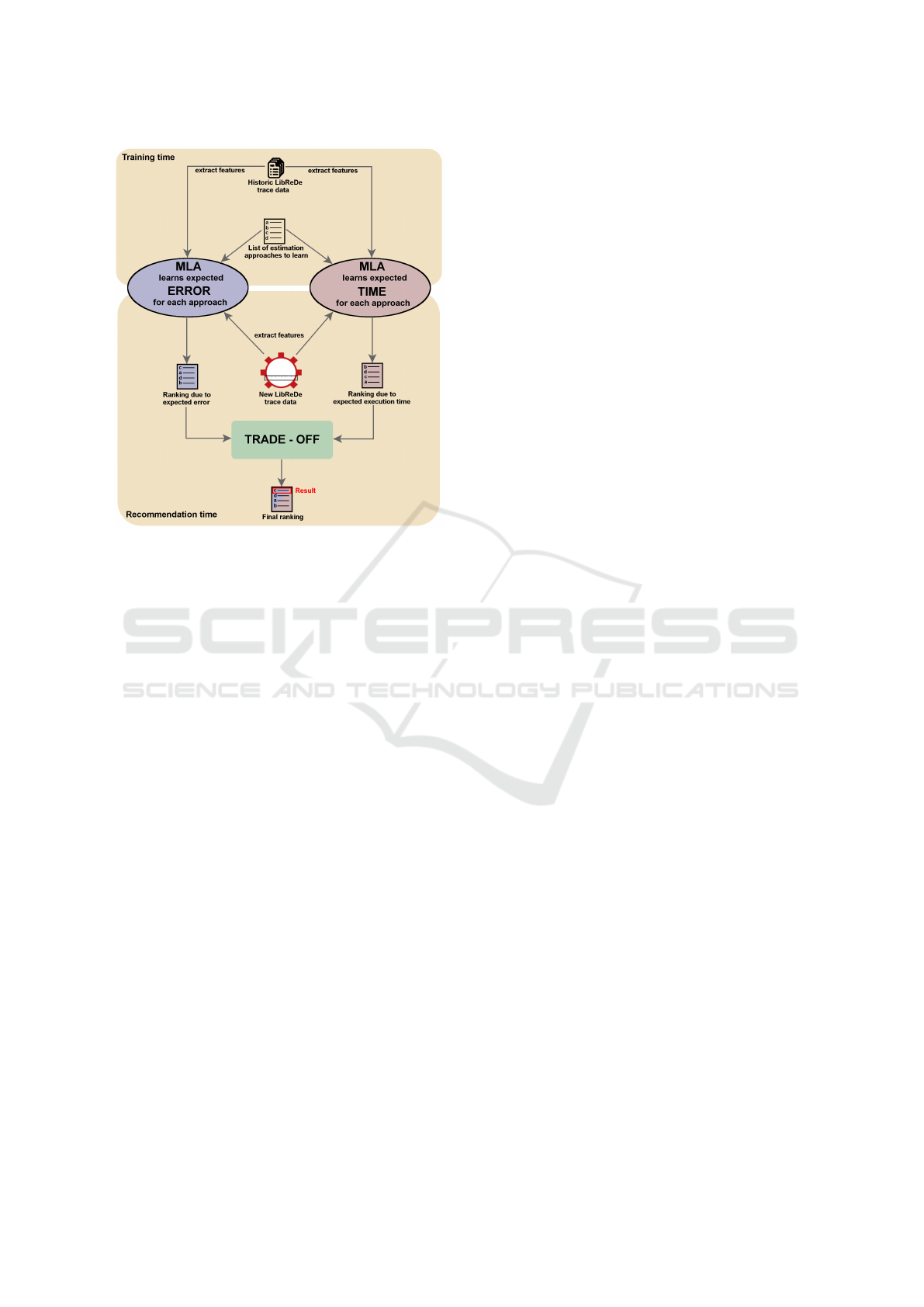
Figure 1: Conceptional overview over the envisioned trade-
off algorithm.
5.1 Trade-off Support
Section 4.2 shows that the best approach in terms
of accuracy is sometimes also the slowest approach.
Therefore, selecting the suitable approach poses a dif-
ferent challenge. What if the slowest approach is too
slow? What if the estimation is needed faster than
a given threshold or the second best (but way faster)
approach might work well enough for a specific sce-
nario?
To tackle this, we want to incorporate a trade-off
algorithm as shown in Figure 1. This algorithm basi-
cally consists of two complementary MLA, basically
regressing or ranking the different approaches by er-
ror and the run-time. (They in turn might consist of
multiple MLAs internally.) After doing so, an arbi-
trary decision process can be inserted to select be suit-
able approach based on the user.
However, this requires that both algorithms are ac-
curate enough to be trustworthy.
5.2 Towards Online SDE Selection
Some other challenges arise, when applying SDE in
an online fashion. As already mentioned in Sec-
tion 3, further questions have to be answered when
live data is incorporated into the training set: What
length should the traces be? How often should the
MLA be retrained? In which intervals should the se-
lection be repeated?
Further technical challenges involve proper par-
allelization (in order to train the MLAs in the back-
ground) as well as memory management and cut-off,
to avoid ever-increasing run-times.
We further plan to include the integration with
our optimization algorithms (Grohmann et al., 2017).
They optimize the parameter configurations based on
a historical data set. Although both approaches can
be used independently from each other, they comple-
ment each other really well. The optimization can
run in parallel to the recommendations and trigger a
retraining, if improved parameter settings have been
found.
6 SUMMARY
This paper introduces the use of Machine Learning
Algorithms in order to recommend or select the best
Service Demand Estimation approach. We develop a
feature set and evaluate the performance of Decision
Trees, Support Vector Machines and Neural Networks
on an offline data set.
The main takeaways are:
• The use of machine learning for the selection of a
Service Demand Estimation (SDE) approach can
improve the estimation time by more than 57%.
The resulting accuracy decrease is less than 0.5%.
• A relatively small set of statistical features is
enough to enable the selection algorithm of pro-
ducing reasonable selections.
• Our experiments show that NN and SVM are ca-
pable of producing excellent result, with NN be-
ing superior in run-time.
• Further work may support a treshold or trade-
off algorithm to recommend the best suitable ap-
proach in a time-critical scenario.
ACKNOWLEDGEMENTS
This work was co-funded by the German Research
Foundation (DFG) under grant No. (KO 3445/11-1)
and by Google Inc. (Faculty Research Award).
REFERENCES
Bauer, A., Herbst, N., and Kounev, S. (2017). Design and
Evaluation of a Proactive, Application-Aware Auto-
Scaler. In ACM/SPEC ICPE 2017.
Using Machine Learning for Recommending Service Demand Estimation Approaches - Position Paper
479

Bause, F. (1993). Queueing petri nets-a formalism for the
combined qualitative and quantitative analysis of sys-
tems. In Proceedings of the 5th International Work-
shop on Petri Nets and Performance Models, pages 14
– 23.
Bolch, G., Greiner, S., de Meer, H., and Trivedi, K. S.
(1998). Queueing Networks and Markov Chains:
Modeling and Performance Evaluation with Com-
puter Science Applications. Wiley-Interscience, New
York.
Breiman, L., Friedman, J., Olshen, R., and Stone, C. (1984).
Classification and Regression Trees. Wadsworth and
Brooks, Monterey, CA.
Brosig, F., Kounev, S., and Krogmann, K. (2009). Auto-
mated Extraction of Palladio Component Models from
Running Enterprise Java Applications. In VALUE-
TOOLS ’09, pages 1–10.
Bryson, A. E. and Ho, Y.-C. (1969). Applied optimal con-
trol : optimization, estimation, and control.
Casale, G., Cremonesi, P., and Turrin, R. (2007). How to
Select Significant Workloads in Performance Models.
In CMG Conference Proceedings.
Casale, G., Cremonesi, P., and Turrin, R. (2008). Robust
Workload Estimation in Queueing Network Perfor-
mance Models. In Euromicro PDP 2018, pages 183–
187.
Cybenko, G. (1988). Continuous valued neural networks
with two hidden layers are sufficient. Technical re-
port, Department of Computer Science, Tufts Univer-
sity, Medford, MA.
Grohmann, J. (2016). Reliable Resource Demand Estima-
tion. Master Thesis, University of W
¨
urzburg.
Grohmann, J., Herbst, N., Spinner, S., and Kounev, S.
(2017). Self-Tuning Resource Demand Estimation. In
IEEE ICAC 2017.
Joanes, D. and Gill, C. (1998). Comparing measures
of sample skewness and kurtosis. Journal of the
Royal Statistical Society: Series D (The Statistician),
47(1):183–189.
Kounev, S., Huber, N., Brosig, F., and Zhu, X. (2016).
A Model-Based Approach to Designing Self-Aware
IT Systems and Infrastructures. IEEE Computer,
49(7):53–61.
Kraft, S., Pacheco-Sanchez, S., Casale, G., and Dawson,
S. (2009). Estimating service resource consumption
from response time measurements. In VALUETOOLS
’09, pages 1–10.
Kumar, D., Tantawi, A., and Zhang, L. (2009). Real-time
performance modeling for adaptive software systems.
In VALUETOOLS ’09, pages 1–10.
Liu, Z., Wynter, L., Xia, C. H., and Zhang, F. (2006). Pa-
rameter inference of queueing models for IT systems
using end-to-end measurements. Perform. Evaluation,
63(1):36–60.
Menasc
´
e, D. (2008). Computing missing service demand
parameters for performance models. In CMG Confer-
ence Proceedings, pages 241–248.
Menasc
´
e, D. A., Dowdy, L. W., and Almeida, V. A. F.
(2004). Performance by Design: Computer Capac-
ity Planning By Example. Prentice Hall PTR, Upper
Saddle River, NJ, USA.
Pacifici, G., Segmuller, W., Spreitzer, M., and Tantawi, A.
(2008). CPU demand for web serving: Measurement
analysis and dynamic estimation. Perform. Evalua-
tion, 65(6-7):531–553.
Rolia, J. and Vetland, V. (1995). Parameter estimation
for performance models of distributed application sys-
tems. In CASCON ’95, page 54. IBM Press.
Rolia, J. and Vetland, V. (1998). Correlating resource de-
mand information with ARM data for application ser-
vices. In Proceedings of the 1st international work-
shop on Software and performance, pages 219–230.
ACM.
Russell, S. and Norvig, P. (2009). Artificial Intelligence:
A Modern Approach (3rd Edition). Prentice Hall, 3
edition.
Sharma, A. B., Bhagwan, R., Choudhury, M., Golubchik,
L., Govindan, R., and Voelker, G. M. (2008). Auto-
matic request categorization in internet services. SIG-
METRICS Perform. Eval. Rev., 36:16–25.
Spinner, S., Casale, G., Brosig, F., and Kounev, S. (2015).
Evaluating Approaches to Resource Demand Estima-
tion. Perform. Evaluation, 92:51 – 71.
Spinner, S., Casale, G., Zhu, X., and Kounev, S. (2014).
Librede: A library for resource demand estimation.
In ACM/SPEC ICPE 2014, ICPE ’14, pages 227–228,
New York, NY, USA. ACM.
Stewart, C., Kelly, T., and Zhang, A. (2007). Exploiting
nonstationarity for performance prediction. SIGOPS
Oper. Syst. Rev., 41:31–44.
Wang, W., Huang, X., Qin, X., Zhang, W., Wei, J., and
Zhong, H. (2012). Application-Level CPU Consump-
tion Estimation: Towards Performance Isolation of
Multi-tenancy Web Applications. In IEEE CLOUD
2012, pages 439 –446.
Wang, W., Huang, X., Song, Y., Zhang, W., Wei, J., Zhong,
H., and Huang, T. (2011). A statistical approach for
estimating cpu consumption in shared java middle-
ware server. In IEEE COMPSAC, 2011, pages 541–
546. IEEE.
Wang, W., P
´
erez, J. F., and Casale, G. (2015). Filling the
gap: A tool to automate parameter estimation for soft-
ware performance models. In Proceedings of QUDOS
2015, pages 31–32, New York, NY, USA. ACM.
Westfall, P. H. (2014). Kurtosis as peakedness, 1905–2014.
rip. The American Statistician, 68(3):191–195.
Zheng, T., Woodside, C., and Litoiu, M. (2008). Perfor-
mance Model Estimation and Tracking Using Optimal
Filters. IEEE TSE, 34(3):391–406.
Zheng, T., Yang, J., Woodside, M., Litoiu, M., and Iszlai, G.
(2005). Tracking time-varying parameters in software
systems with extended Kalman filters. In CASCON
’05, pages 334–345. IBM Press.
CLOSER 2018 - 8th International Conference on Cloud Computing and Services Science
480
