
Industrial Optimal Operation Planning with Financial
and Ecological Objectives
Camille Pajot
1
, Benoit Delinchant
1
, Yves Maréchal
1
, Fredéric Wurtz
1
, Lou Morriet
1
,
Benjamin Vincent
2
and François Debray
2
1
Univ. Grenoble Alpes, CNRS, Grenoble INP*, G2Elab, 38000 Grenoble, France
2
CNRS, LNCMI, F-38000 Grenoble, France
{benjamin.vincent, francois.debray}@lncmi.cnrs.fr
Keywords: Energy Planning, MILP Optimization, District, Energy Efficiency, Co
2
Emissions.
Abstract: As energy transition is fundamental to have a chance to fight climate change, every stakeholder concerned
by energy should be able to get a better knowledge of the consequences of these actions. However, it could
be very complex to understand energy problematics without being an expert. This article focuses on giving
the possibility to an energy intensive consumer of a district to make decisions about its energy planning
while taking into account its specific operating constraints. A practical case has been studied in a heat
recovery project to help the experiments planning of a research laboratory according to the thermal needs of
the district. At first, the energy planning only aims to reduce its electricity consumption bill. In a second
time, we consider re-using the thermal power from processes cooling. Then, two energy planning were
realised: reducing district CO
2
emissions and reducing district supply cost. Finally, trade-offs between these
two goals have been studied. The work is based on mixed-integer linear optimization models (MILP)
gathered into a Python library to provide a modular decisions tool for energy stakeholders.
1 INTRODUCTION
More and more modeling approaches and tools
emerge for the district-scale energy systems
(Allegrini et al., 2015). However, district energy
models focus more on simulation or design
optimization (Schütz .et al., 2016) than on energy
management optimization. Our objective was to
develop an optimization tool to help energy
stakeholders to make decisions about district energy
management with technical, financial,
environmental and social aspects.
Lots of the emerging district tools are based on a
bottom-up methodology gathering thermal buildings
models to create a district one (Lauster et al., 2014),
(Jimeno et al., 2015) while we aim to create a single
multi-energies representation with production,
conversion and consumption.
Before the district scale, energetic optimisation
has been studied at the urban level through lots of
optimization techniques (Keirstead et al, 2012), (Z.
Shi et al., 2017). Best et al. provide genetic
optimization models for supply and demand of
heating, cooling, and electricity (Best et al., 2015),
while Shabanpour-Haghighi et al. use heuristic
algorithm through the modified teaching–learning
based optimization (MTLBO) in order to minimize
the fuel cost in multi-carrier energy network
(Shabanpour-Haghighi et al., 2015
). Finally, a lot of
them preferred a Mixed Integer Linear Programming
(MILP) approach, as B. Morva et al. who optimized
both design and operational aspects of an urban
energy system (Morva et al, 2016).
In our study, several objectives will be presented:
reducing an energy supply bill, reducing CO
2
emissions of a district and reducing the heating
supply cost of a district. Therefore, the presented
problems require a formulation of energetic,
economic and CO
2
flux, what generates hundreds of
variables. In order to easily deal with a large amount
of variables, we are working on MILP formulation.
214
Pajot, C., Delinchant, B., Maréchal, Y., Wurtz, F., Morriet, L., Vincent, B. and Debray, F.
Industrial Optimal Operation Planning with Financial and Ecological Objectives.
DOI: 10.5220/0006705202140222
In Proceedings of the 7th International Conference on Smart Cities and Green ICT Systems (SMARTGREENS 2018), pages 214-222
ISBN: 978-989-758-292-9
Copyright
c
2019 by SCITEPRESS – Science and Technology Publications, Lda. All rights reserved

2 INDUSTRIAL ENERGY
PLANNING TO MINIMIZE
ENERGY SUPPLY BILL
For industries and other energy intensive users, the
energy bill strongly affects their operation. From
simple operation schedules based on lower prices to
energy management policies, planning the energy
repartition to stay competitive becomes crucial.
In France, Energy Intensive Industries (EII) such
as steel, chemical and microelectronics’ industries or
paper mills can be directly connected to the
transmission system (Rte&Vous Le Mag, 2018). In
this case, electrical access and supply are two
separated contracts. With temporal repartition of
prices at several scales, the associated pricing is
more complex than a simple electrical cost for
standard consumer (Clients.rte-france.com, 2018).
At its Grenoble site, the National High Magnetic
Field Laboratory (LNCMI) offers static magnetic
fields up to 36 T, thanks to several magnets supplied
by a 24 MW electrical power station (LNCMI,
2017). The mean consumption during a day of
experiment is 6 MW (one fourth of the maximum
value), while the annual consumption for this
laboratory is typically around 14 GWh leading to an
important electricity bill. This should be taken into
account when experiments on magnetic fields are
planned, task which is currently handled manually.
Our study case focuses here on minimizing the
electricity bill considering specific operating
constraints and complex pricing structure.
2.1 Energy Pricing for Energy
Intensive Industries
2.1.1 Pricing Structure for French Electrical
Transmission System Access and
Supply
As explained before, EIIs have direct access to the
electrical transmission network. For those, electricity
access is not included into the supply and requires
subscribing two different contracts:
• The TURPE: French price for accessing
the public transmission system of
electricity
• An electrical supply contract
The TURPE pricing for LNCMI has an hourly-
seasonal structure (price variations at different time
scales: seasonal to hourly), which can be presented
as follows (Table 1).
In our study, only the three major components of
the price have been modeled: the power part
(subscription), the energy part and the taxes (see
equations 1, 2 and 3 below).
Power_part : b
k
= b
1
* Ps
1
+ ∑
k>1
b
k
(Ps
k
-Ps
k-
1
)
(1)
Energy_part : c
k
= ∑
k
c
k
E
k
(2)
Total electricity cost = Power_part +
Energy_part + Taxes
(3)
Moreover, according to the TURPE, the
subscribed power has to respect the following rule:
Ps
k
≤ Ps
k+1.
(Clients.rte-france.com, 2018)
Table 1 : TURPE 4 pricing structure.
Time
period
b
k
[€/kW/y
]
c
k
[c€/kWh]
Monthly
period
Day type Hour range
k=1
9.24
3.01
Dec., Jan., Feb.
Working
9:00-10:59 / 18:00-19:59
k=2 8.5932 2.73 Dec., Jan., Feb. Working
7:00 - 8:59 / 11:00 – 17:59
20:00 - 22:59
k=3
6.6528
2.26
March, Nov.
Working
7:00– 22:59
k=4
5.1744 1.59
Dec., Jan., Feb.
Working
0:00 - 6:59 / 23:00 – 23:59
Non-working 0:00 – 23:59
k=5 4.2504 1.22 March, Nov.
Working
0:00 – 6:59 / 23:00 – 23:59
Non-working
0:00 – 23:59
k=6 3.696 1.37
Ap., May, June,
Sept., Oct.
Working 7:00– 22:59
k=7 1.9404 0.86
Ap., May,
June, Sept.,
Oct.
Working
0:00 - 6:59 / 23:00 – 23:59
Non-working 0:00 – 23:59
k=8
0.924
1.08
July, August
All
0:00 – 23:59
Industrial Optimal Operation Planning with Financial and Ecological Objectives
215

Where:
b
k
:
Price for the capacity defined by time
interval k and the tariff version
Ps
k:
Subscribed power for time interval k
c
k:
Price for the energy for time interval k and
the tariff version concerned
E
k
:
Active energy extracted over the year during
time interval k, expressed in kWh
Energy supply prices are based on electrical
consumption forecasts for each price period (same
pricing repartition as TURPE). This contractual
commitment forces the LNCMI to estimate its
electrical load repartition by time period one year
ahead explaining the energy planning need for an
entire year. As mentioned before, this work is
realised by a member of the LNCMI, who could
benefit from the developed tool.
2.1.2 Operation Constraints
Each big consumer has its own operating
constraints: some industries cannot ever stop their
process, whereas some others can only operate on
working days for instance. Understanding and being
able to describe these particulars needs is very
important to get a plausible energy planning.
Therefore, a part of our work was to translate
common constraints into easy Python objects and
thus enrich the possibilities of the decision tool.
As an industry, LNCMI has operating
constraints. In its case, it is estimated that it cannot
handle experiments more than 16 hours per day
(considering for instance the time required between
experiments). Moreover, the laboratory is closed
several days per year (two weeks starting at
Christmas’ Eve) and should be working all other
days.
On the other side, quality of life at work is
currently taken into account without being strictly
formalized, by avoiding too many nights and
weekends of work. To do so, the current planning is
created with energy limits on the corresponding time
periods. For instance, maximum values are fixed for
some time periods including nights and non-working
days as k=4, k=5 and k=7.
In our study, to avoid an experiment planning
only focused on electricity prices, these current
energy limits will be directly translated into
optimization constraints (see equations 5 to 8).
2.2 Optimization Problem Formulation
2.2.1 Daily Steps Model
For a yearly study, an hourly step could lead to
heavy formulations due to the amount of decision
variables. To avoid computational issues in case of
complex problems, we went for a daily step when
we aim to optimize an annual energy planning.
However, as the price may change during the
day, we expressed the daily energy consumption as
consumption at a fixed equivalent power and
deducted the equivalent operating hours, according
to equation 4.
op
h
(t) = e
in
(t) / p
eq
(t)
(4)
This deduction of an equivalent number of
operating hours is fundamental to evaluate the
consumption cost of the day, taking intra-day prices
variation into account. Indeed, LNCMI expenses are
calculated as follows:
expense
lncmi
(t) = p
eq
∑
k
c
k
* op_h
k
(t)
(5)
∑
k
op_h
k
(t) = op
h
(t)
(6)
Where:
e
in
(t):
Electrical consumption for the day t
p
eq
:
Equivalent power of the LNCMI
(6MW)
op
h
(t):
Equivalent number of operating hours
for the day t
op_h
k
(t):
Number of operating hours at price c
k
for the day t
2.2.2 Translation of Operating Constraints
into Energetic Constraints
According to the use of the magnets, each
experiment led in the LNCMI consumed a different
amount of electricity. By knowing by advance the
experimentations planned on the following year, it
becomes possible to evaluate the annual electrical
consumption to come. For the year 2107, it has been
estimated at 14 GWh, leading to equation 7:
∑
t
e
in
(t) = 14000000 for t in {0; 364}
(7)
As written before, the LNCMI closes annually
for two weeks, but the installation is working all the
others days with a minimal value of 0.5 hours per
day, leading to the equations 8 and 9. The minimal
value of 0.5 daily operating hours has been set from
an energetic point of view, forcing the installation of
consuming at least 3MWh per day (see equation 4).
SMARTGREENS 2018 - 7th International Conference on Smart Cities and Green ICT Systems
216
e_in
lncmi
(t) = 0 for t in annual closure
(8)
op_h
lncmi
(t) ≥ 0.5 for t not in annual closure
(9)
Finally, the next equations translate LNCMI
choices to avoid high electricity prices, while
considering the quality of life at work. Indeed, the
equation 9 expresses the fact that no power
subscribing was taken for time periods tp
1
and tp
2
, in
order to limit energy costs and avoid a bill increase.
In the other hand, as explained in 2.1.2, quality of
life at work is considered into the energy planning.
Limits are fixed in terms of energy minimums
or/and maximums for some pricing time periods and
are based on the LNCMI experience. If we call tp
k
the time period corresponding to the TURPE period
at price c
k
, the constraints are expressed as follows
in equations 10, 11, 12 and 13.
∑
t
e
in
(t) = 0 for t in tp
1
and tp
2
(10)
∑
t
e
in
(t) ≤ 2000 for t in tp
4
(11)
∑
t
e_in
lncmi
(t) ≥ 500 for t in tp
3
(12)
∑
t
e
in
(t) ≤ 1500 for t in tp
5
(13)
∑
t
e
in
(t) ≤ 6600 for t in tp
7
(14)
2.2.3 Objective Formulation
In this case study we aim to reduce the LNCMI
electricity bill by optimizing its consumption
planning under specific constraints. The expressions
of these constraints were expressed above, so that
the objective formulation is:
Minimize ( ∑
t
expense
lncmi
(t) )
(15)
With expense
lncmi
expressed in equation 5.
2.3 Results
2.3.1 Optimal and Previous Planning
Comparison
The current LNCMI energy planning is based on a
compromise between consuming low prices
electricity and avoiding too many working nights
and weekends. To allow a comparison between
optimal and usual planning (created manually),
values chosen for the 2017 year are shown in the
second column of Table 2. The energetic values are
expressed in MWh, while the electricity prices have
been normalised regarding to the maximal value for
a confidentiality purpose.
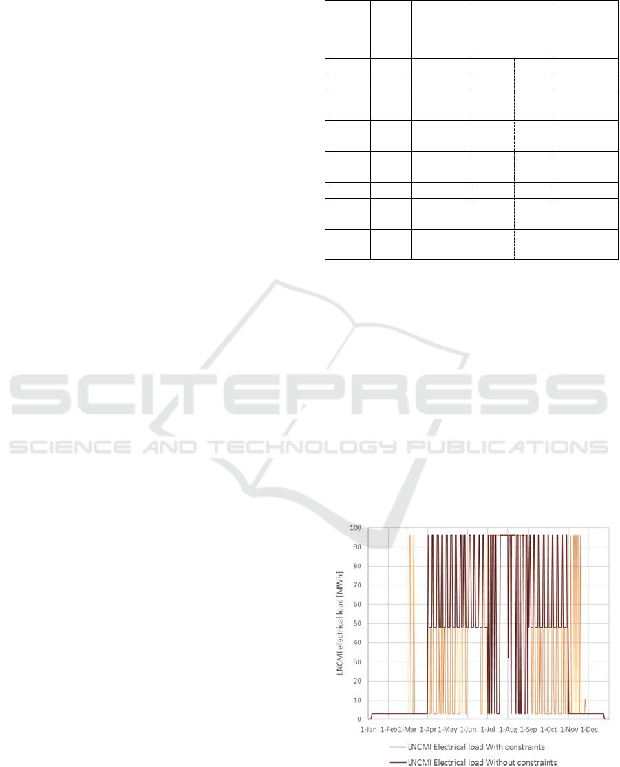
Table 2: Comparison between current and optimized
LNCMI energy planning.
Time
perio
d
Elec.
price
[pu]
2017
Planning
Optimization
Results
Constraints
Results
without
constraint
s
1
1.00
0
= 0
0
0
2
0.98
0
= 0
0
0
3
0.83 180
≥
500
500 0
4
0.65 1 200
≤
2000
234 234
5
0.56 1 420
≤
1500
714 183
6
0.67
250
None
0
0
7
0.48 6 600
≤
6600
660
0
9648
8
0.55 4 350 None
595
2
3935
As a first approach, we considered the
optimization problem as a minimization of the
electricity bill under constraints. Energetic planning
for this optimization can be found in the fourth
column next to the energetic constraints taken into
account (equations 9 to 13). We can notice that some
of the constraints are reached (see values in red), so
that we can hope to get better results in terms of
electrical bill reduction if we relax the constraints.
These results led us to the second approach,
without the energetic constraints put in place
manually, but not corresponding to a real constraint
of the installation, in opposite to the annual closure
for instance. Results of this optimization are shown
in the last column of Table 2 and Figure 1.
Figure 1: LNCMI electrical consumption from
optimization results.
Industrial Optimal Operation Planning with Financial and Ecological Objectives
217

These values complete results from the first
approach, by giving several indications as:
• As suspected, forcing the electrical
consumption to zero for the first two price
periods is not necessary because of high
prices.
• Relaxing the two periods where limits are
reached can significantly change the energy
repartition.
For a better understanding of the impact of the
relaxation of energy limitations, we will focus on the
objective, which is the LNCMI electricity bill
reduction.
In the first approach, the bill reduction with the
new energy planning is estimated of 0.4%. Even if
this diminution seems low, we have to keep in mind
that our problem is more constrained than the
current energy planning. Indeed, it has been wished
that at least 500 MWh would be planned during the
fourth time period, while only 180 MWh are
currently planned. In the second approach, the bill
reduction reaches 4.6%, but the impact on working
conditions is not taken into account, as we relaxed
the associated constraints.
2.3.2 Conclusion and Prospects
The energy planning of an EII allows us to use its
consumption flexibility to adjust its operation.
Moreover, it could also help the consumer to
identify which constraints are the more restrictive
from an economic point of view. However, it is
important to keep in mind what impact could have
the relaxation of restrictive constraints (less working
quality in our case).
It has been shown that this first modeling could
be used to minimize the energy bill with a defined
pricing, but we can also imagine using it to compare
financial gains associated with different energy
supply contracts. Nevertheless, these two
applications have as sole goal to serve economical
interest of one particular actor, while we could
imagine considering other goals.
A prospect for this decision tool could be to
explicitly quantify the social impact of energy
planning to realise multi-objectives optimizations
and to help to choose a compromise between these
two interests. Another one would be to use this
flexibility into more ambitious projects and serve
general interest at district scale.
3 COMBINED OPTIMIZATION
OF ENERGY CONSUMPTION
AND DISTRICT HEATING
On the one hand, for lots of energy experts, energy
efficiency will be one of the keys of a successful
energy transition (Smartgrids-CRE, 2017), so that
energy losses reduction becomes more and more
important. On the other hand, Joule losses in
industrial processes can lead to temperature
problems and lots of EIIs are forced to put in place
cooling installations to evacuate generated heat. One
way of reducing our total energy consumption
consists in the heat losses re-use to supply heating
demand instead of simply trying to evacuate it.
Well-known examples are datacenters (ADEME,
2015), but it could be achieved on the LNCMI
installation with its annual consumption of 14 GWh
and its cooling installation (which evacuates almost
12 GWh of heat). Therefore re-using calories from
LNCMI magnets cooling to complete the heat
supply of a district (annual load of 21GWh) instead
of dissipating it into the neighbour river is studied in
the project Valocal (C. Pajot et al., 2017).
3.1 Carbon Footprint for Heating
Supply
Our first case study aims to reduce the carbon
footprint of a district by minimizing the CO
2
emission generated to cover the heat load of
buildings connected to a heating network. This
reduction of greenhouse gases emissions will be
realised thanks to the choice to solicit either the
electrical network or the heating network offer by
re-using LNCMI Joule losses.
3.1.1 Energetic Model
Indeed, from an energetic point of view, the LNCMI
could be considered as a conversion unit between
electricity and heat with a conversion rate depending
of temperature conditions. To simplify the problem
and focus on power flows only, we modeled the
LNCMI process with a fixed electrical to thermal
conversion rate of 85% (mean value of thermal
losses observed in real conditions).
e_out
LNCMI
(t) = 0.85 * e_in
LNCMI
(t)
(16)
The previous operating constraints were kept and
a thermal dissipation model was added as a flexible
consumption (see Figure 2). Heating power provided
by the LNCMI can be either dissipated through this
SMARTGREENS 2018 - 7th International Conference on Smart Cities and Green ICT Systems
218
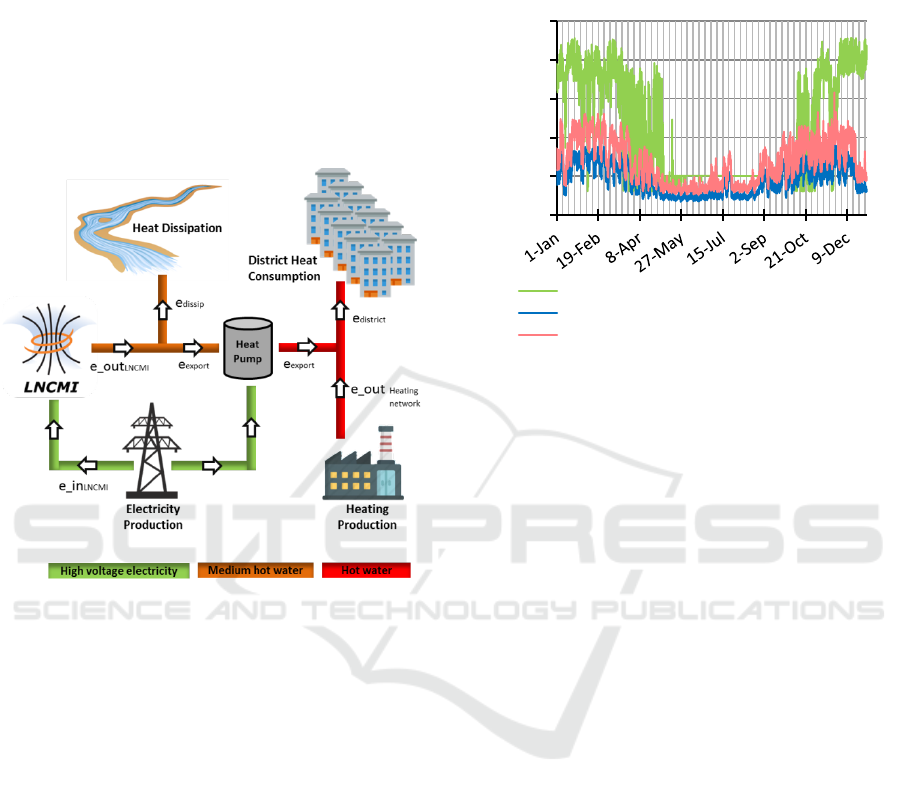
flexible consumption unit or exported to the heating
network as expressed in equation 16:
e_out
lncmi
(t) = e
dissip.
(t) + e
export
(t)
(17)
e
export
: export to the district heating network
e
dissip
: the variable dissipated heat
The energy networks (heating and electrical)
were modeled as production units with limitations
on maximal power delivered corresponding to
network maximal power flux.
Figure 2 : Schematic diagram for district energetic model.
In our study case, we don’t consider the
possibility of load variations (load shifting, load
reduction, etc.), so that the district heating
consumption was modeled as a fixed load
corresponding to a representative year.
3.1.2 Environmental Model
3.1.2.1 French Electrical Emissions
The French electrical system is well known for its
low CO
2
emission, due to its high share of nuclear
power (72% of the 2016 electrical production (RTE,
(2016)). Moreover, this massive nuclear power
integration into the electrical mix has affected the
heating sector with one of the highest electrical
heating share among European countries, so that
fossil fuel production units are only started to
provide supply for load peaks (see French electricity
network CO
2
emission during a year in Figure 3).
That is why we decided to study the subject of
energy carbon footprint from a dynamic point of
view (ADEME, 2014).
For both of the production units modelling
energy networks, a dynamic CO
2
emission rate was
defined corresponding to the daily mean value (see
‘Electricity’ and ‘Heat’ curves on Figure 3).
Figure 3: Dynamic CO
2
emission from energetic
(electrical and heat) production.
3.1.2.2 Additional emissions
Moreover, temperature levels need to be increased to
reach those of the heating grid. Therefore, the
resulting electrical consumption increase needed to
feed a heating pump was also considered. As before,
we consider temperature variations to be negligible
and make the hypothesis of a constant ratio. After a
technological benchmark realised in the Valocal
project, the heat pump was chosen with a coefficient
of performance equal to 3.25.
Therefore, if we consider the CO
2
emissions
related to the entire conversion chain of electrical
consumption into heat production, we have to add
the CO
2
emission from the electrical consumption of
the heat pump to the electrical consumption to the
LNCMI electrical consumption converted into heat
and exported into the heating network.
For each thermal kWh exported, 1/0.85 electrical
kWh was consumed by the LNCMI and an extra
1/3.25 electrical kWh was consumed by the heat
pump leading to an equivalent CO
2
emission rate
(see ‘Electricity conv. into heat by LNCMI’ on
Figure 3) expressed as follows:
co
2eq rate
(t) = co
2elec rate
(t) * (1/0.85 + 1/3.25)
(18)
For reminder, the objective in this case study is
to reduce the carbon footprint of the district by
minimizing the CO
2
emission of the heating
network. To simplify, we introduced an equivalent
CO
2
emission rate (equation 16) for thermal energy
provided by LNCMI cooling system, so that
0
50
100
150
200
250
CO2 emissions [g/kWh]
Heating network
French electrical network
Electricity conv. Into heat by LNCMI
Industrial Optimal Operation Planning with Financial and Ecological Objectives
219
objective can be formulated as:
Minimize ∑
t
CO
2district
(t)
(19)
Where: CO
2district
(t) = co
2eq rate
(t) * e
export
(t)
+ co
2heat rate
(t) * e_out
heating network
(t)
(20
)
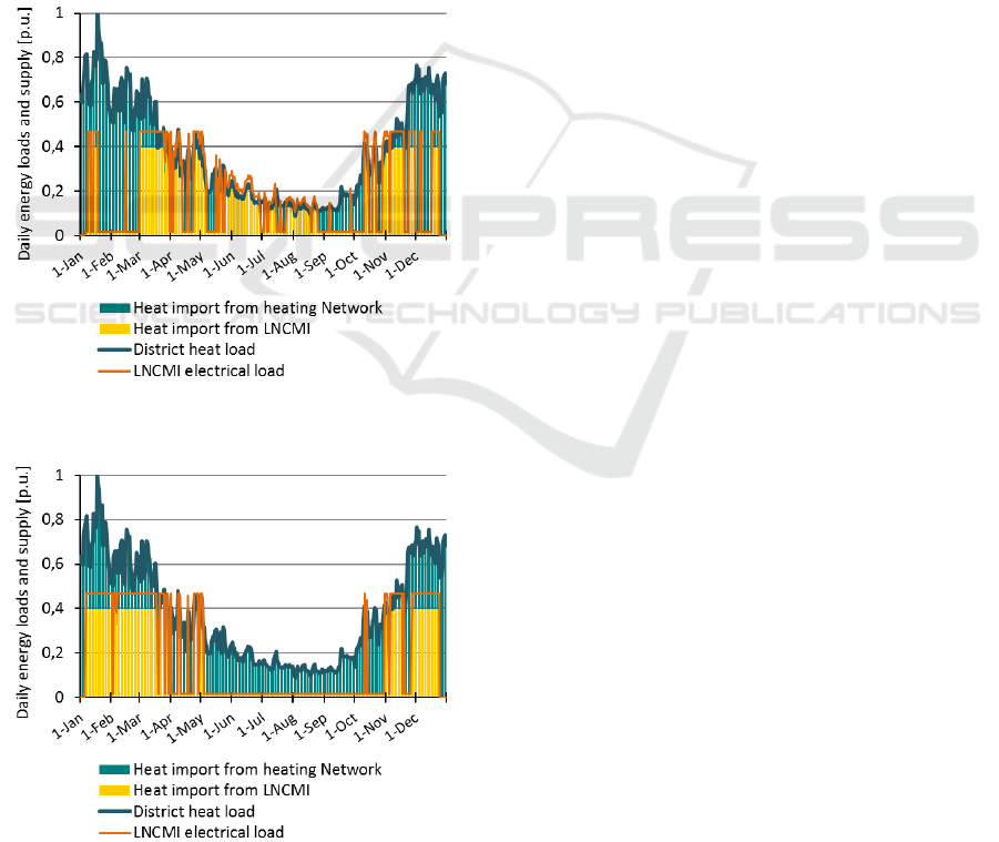
3.1.3 Results and Prospects
As before, we studied two different approaches: with
and without LNCMI energy limitation constraints.
We reached a reduction of CO
2
emission of 28% in
the first case and 35% in the second case.
Unlike the energy bill reduction problem, we can
notice that energy limitations are less restrictive in
order to minimize CO
2
emission. However, the
energy repartition changes a lot between
optimizations with or without energy limitations (see
Figure 4 and Figure 5).
Figure 4: District energy flows repartition with LNCMI
constraints taken into account.
Figure 5: District energy flows repartition without LNCMI
constraint.
In section 2, we optimized energy planning in
order to reduce the electricity bill and demonstrated
that the currently used energy planning was already
a good optimization as we reduced the bill with and
without energy constraints of respectively 0.4% and
4.6%. This first case aimed to help a single
stakeholder, while we focused on the global interest
through an ecological optimization in 3.1.
Nevertheless, we can now wonder how the
LNCMI is impacted by these ecological
considerations. In the first case, the electricity bill of
the LNCMI increases by 21% and reaches 39% of
raise when we remove the LNCMI energy
limitations. In these cases, why would the LNCMI
be the one to pay the CO
2
emissions reduction?
Moreover, the electricity cost to feed the heat pump
was not included into the increases, while some
stakeholders would have to pay for it.
These results raise an issue: how to guarantee no
economic effect on the heating consumer bill, while
guaranteeing no LNCMI electricity bill increase
either?
3.2 Reduction of a District Heating
Supply Cost
One of the main issues in energy transition is to
mitigate our environmental impact without leading
to an uncontrolled raise of energy prices for the
consumer. How to do so, when we have the
possibility to produce at low price with energies as
coal with a strong impact on global warming for
instance?
That is the problem we address in this last case
study at a district scale. Our aim is to add a financial
modeling to our previous case study to find
compromises between ecologic and economic points
of view.
3.2.1 Financial Model
We found previously that LNCMI electricity bill
could increase when we reduced the CO
2
emission.
However, we did not define any economic model to
compensate this bill augmentation.
Here, we decided not to model the financial
transactions between the heat supplier and the
LNCMI to keep all types of remuneration possible.
To do so, we considered the LNCMI as a heating
production unit with an energy production cost.
The production cost of 1 thermal kWh is
estimated as the electrical consumption cost of the
heat pump added to the increase of LNCMI bill
regarding to the current one. LNCMI expense model
SMARTGREENS 2018 - 7th International Conference on Smart Cities and Green ICT Systems
220
is usable for any energy unit connected to the
transmission grid under the condition of providing
an equivalent power of consumption. Nevertheless,
applying this particular point to the heat pump could
lead to an over-estimation of its electricity
consumption cost. We preferred here an average
approach as studied on the ecological study case,
with a mean dynamic cost of electricity.
3.2.2 Which Trade-off between Divergent
Interests?
Optimization focused on district energy heating cost
only can lead to a reduction of 8.3% with the
LNCMI energy limitations. This result seems to say
that we get a margin to lower the CO
2
emission of
the district without increasing energy cost for the
consumer. Our last case study aims to verify this
assumption.
For this purpose, we combine financial and
ecological objectives into a single one as follows
with a coefficient α to weight the objectives:
Minimize:
α ∑
t
CO
2district
(t) / CO
2max
+
(1-α) ∑
t
Ct
district
(t) / Ct
max
(21
)
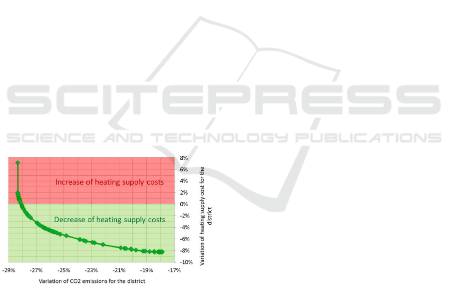
Results obtained with α-values in [0; 1] showed
that with great use of LNCMI flexibility, we could
achieve both of the goals previously set: CO
2
emission reduction and heating supply cost
reduction (see the Pareto diagram Figure 7).
Figure 6: Pareto diagram for CO2 emission and heating
supply bill reduction.
The abscissa shows the impact on CO
2
emission
compared to the current estimation, while the y-axis
represents the financial objective with the variation
of heating supply cost (positive values when cost
increases and negative ones when it decreases). We
can observe on the Figure 6, the two extreme points
corresponding to each objective. When alpha equals
0, the optimization is only financial and we reach the
8.3% of savings announced before. In the other
hand, when alpha equals 1, we recognized the 28%
of CO
2
emission reduction from the environmental
optimization in 3.1.
If we consider only the results leading to supply
cost decreases, we can see that reducing CO
2
emissions is possible without increasing the energy
supply and can even lead to supply savings.
However, these savings do not consider the
investment costs to re-use the LNCMI thermal
losses. That is why one of the outlooks for the use of
this decision tool could be the study of return of
investment in the case of heat recycling.
4 CONCLUSIONS
To summarize, we have shown that the developed
decision tool could serve several needs:
• Reducing its energy supply bill under
operation constraints
• Reducing the CO
2
emission of a district
• Reducing the heating supply cost of a
district
With the defined energy limitations, the LNCMI
optimal planning can only reduce by 0.4% the
amount of the energy bill, while this decrease
reached 4.8% when relaxing these limitations.
A multi-objective approach could be studied to
take into consideration both of the financial and
working quality aspect, by adding a social modeling.
Moreover, the LNCMI energy planning could serve
more ambitious projects than only bill reduction as
the Valocal project, which aims to re-use LNCMI
heat losses for building heating.
In this scenario, two goals have been studied
(financial and ecological). Regarding the ecological
optimization, the reduction of CO
2
emissions can
reach 35% and heating supply cost can decrease by
8.8% for a financial optimization. Finally, we have
seen that both goals could be achieved by merging
the two objectives into one.
ACKNOWLEDGEMENTS
The VALOCAL project was funded by the CNRS
Interdisciplinary Mission (MI-CNRS) with support
from the Institute of Sciences and Engineering and
Systems (INSIS-CNRS). The authors thank these
authorities, which have made possible through this
funding to initiate transdisciplinary work on an
Industrial Optimal Operation Planning with Financial and Ecological Objectives
221

original issue of energy optimization.
This work is supported by the French National
Research Agency in the framework of the
"Investissements d'avenir" program (ANR-15-
IDEX-02).
REFERENCES
Allegrini, J., Orehounig, K., Mavromatidis, G., Ruesch, F.,
Dorer, V. and Evins, R. (2015). A review of modelling
approaches and tools for the simulation of district-
scale energy systems. Renewable and Sustainable
Energy Reviews, 52, pp.1391-1404.
Schütz, T., Schiffer, L., Harb, H., Fuchs, M. and Müller,
D. (2017). Optimal design of energy conversion units
and envelopes for residential building retrofits using a
comprehensive MILP model. Applied Energy, 185,
pp.1-15.
Lauster, M., Teichmann, J., Fuchs, M., Streblow, R. and
Mueller, D. (2014). Low order thermal network
models for dynamic simulations of buildings on city
district scale. Building and Environment, 73, pp.223-
231.
Jimeno, A. S., Fonseca, A., 2015. Integrated model for
characterization of spatiotemporal building energy
consumption patterns in neighborhoods and city
districts, Applied Energy, 142, pp.247-265.
Keirstead, James, Jennings, Mark, Sivakumar, Aruna,
2012. A review of urban energy system models:
approaches, challenges and opportunities. Renewable
and Sustainable Energy Reviews, 16, pp. 3847-3866.
Shi, Zhongming, Fonseca, Jimeno A., Schlueter, Arno,
2017. A review of simulation-based urban form
generation and optimization for energy-driven urban
design, Building and Environment, 121, pp.119-129.
Best, Robert E., Flager, Forest, Lepech, Michael D. , 2015.
Modeling and optimization of building mix and energy
supply technology for urban districts, Applied Energy,
159, pp.161-177.
Shabanpour-Haghighi, Amin, Seifi, Ali Reza, 2015.
Simultaneous integrated optimal energy flow of
electricity, gas, and heat, Energy Conversion and
Management, 101, pp.579 – 591.
Morvaj, Boran, Evins, Ralph, Carmeliet, Jan, 2016.
Optimising urban energy systems: Simultaneous
system sizing, operation and district heating network
layout, Energy, 116, pp.619-636.
Rte&Vous Le Mag. (2018). 258 entreprises directement
connectées au réseau RTE : des enjeux XXL. [online]
Available at: http://lemag.rte-et-vous.com/dossiers/
258-entreprises-directement-connectees-au-reseau-rte-
des-enjeux-xxl.
Clients RTE-France. (2016). TURPE 4 : Tarification des
réseaux. [online]. Available at: https://clients.rte-
france.com/htm/fr/mediatheque/telecharge/Comprendr
e_le_tarif_01_08_2016.pdf.
LNCMI. (2017), Laboratoire National des Champs
Magnétiques Intenses [online]. Available at:
http://lncmi.cnrs.fr/spip.php?rubrique17&lang=fr.
Smartgrids-CRE. (2017) L’efficacité énergétique, un
principe structurant de la transition énergétique
[online]. Available at: http://www.smartgrids-
cre.fr/index.php?p=efficacite-energetique.
ADEME. (2015), La chaleur fatale industrielle.
Pajot, Camille, Delinchant, Benoit, Marechal, Yves,
Wurtz, Frédéric, Debray, François, Vincent, Benjamin.
2017. Valorisation optimale de chaleur fatale d'un site
à très forte consommation électrique, Conférence des
Jeunes Chercheurs en Génie Electrique (JCGE),
Arras.
RTE, (2016), Statistiques de production, consommations
et échanges. [online] Available at: http://www.rte-
france.com/fr/article/statistiques-de-l-energie-
electrique-en-france.
ADEME, (2014), Documentation des facteurs d'émissions
de la Base Carbone. [online] Available at:
http://www.bilans-
ges.ademe.fr/static/documents/[Base%20Carbone]%20
Documentation%20g%C3%A9n%C3%A9rale%20v11
.0.pdf.
SMARTGREENS 2018 - 7th International Conference on Smart Cities and Green ICT Systems
222
