Computer-aided Formal Proofs about Dendritic Integration

within a Neuron

Oph

elie Guinaudeau

, Gilles Bernot

, Alexandre Muzy

, Daniel Gaff

and Franck Grammont

Universit

e C

ote d’azur, CNRS, I3S, France

Universit

e C

ote d’azur, CNRS, LEAT, France

Universit

e C

ote d’azur, CNRS, LJAD, France

Keywords:

Single Neuron Modelling, Dendrites, Signal Integration, Formal Methods, Model Checking.

Abstract:

This article is threefold: (i) we deﬁne the ﬁrst formal framework able to model dendritic integration within

biological neurons, (ii) we show how we can turn continuous time into discrete time consistently and (iii) we

show how a Lustre model checker can automatically perform proofs about neuron input/output behaviours

owing to our framework.

Our innovative formal framework is a carefully deﬁned trade-off between abstraction and biological relevance

in order to facilitate proofs. This framework is hybrid: inputs entering the synapses as well as the soma output

are discrete signals made of spikes but, inside the dendrites, we combine signals quantitatively using real

numbers. The soma potential is inevitably speciﬁed as a differential equation to keep a biologically accurate

modelling of signal accumulation. This prevents from performing simple formal proofs. This has been our

motivation to discretize time. Owing to this discretization, we are able to encode our neuron models in Lustre.

Lustre is a particularly well suited ﬂow-based language for our purpose. We also encode in Lustre a property of

input/output equivalence between neurons in such a way that the model checker Kind2 is able to automatically

handle the proof.

1 INTRODUCTION

Many studies suggest that there is a strong interdepen-

dence between morphology and information process-

ing capabilities of a neuron (Bianchi et al., 2012; Mo-

han et al., 2015; Hu and Vervaeke, 2017). In this pi-

oneering work, we make use of formal methods from

computer science to investigate how single neurons

process information, with a particular emphasis on

their dendritic morphology.

Neurons are the building blocks of the brain.

They are highly connected and communicate through

electrical impulses. Typically, neurons receive those

signals on branched extensions called dendrites, at

speciﬁc locations named synapses (Figure 1). All

the stimuli are ﬁnally integrated at the soma. If the

resulting signal accumulation is strong enough, it is

transmitted to neighbouring neurons through the axon

which is another kind of extension. There are many

types of neurons (Mel, 1994; Stuart et al., 2016)

and some of them are structurally and functionally

very different from the standard one described above,

depending on the respective sizes on the constituting

Figure 1: Schematic representation of a standard biological

neuron.

sub-parts.

There can be between a few to several tens thou-

sands of synapses as a result of the connectivity

level of the neuron. The incoming signals interact

continually in time and space and while propagat-

ing through the dendrites towards the soma, signals

are signiﬁcantly modiﬁed. Indeed, many parame-

ters of information-processing such as signal ﬁltering,

response speed and connectivity, are strongly inﬂu-

enced by the dendrites properties (Williams and Stu-

Guinaudeau, O., Bernot, G., Muzy, A., Gaffé, D. and Grammont, F.

Computer-aided Formal Proofs about Dendritic Integration within a Neuron.

DOI: 10.5220/0006680500490060

In Proceedings of the 11th International Joint Conference on Biomedical Engineering Systems and Technologies (BIOSTEC 2018) - Volume 3: BIOINFORMATICS, pages 49-60

ISBN: 978-989-758-280-6

art, 2002; Stuart et al., 2016). Therefore, it makes this

sophisticated structure a key determinant of neuronal

computation.

A combination of experimental and theoretical

work is required to make the link between structure

and function of neurons. Nowadays and despite re-

cent advances, dendrites are still difﬁcult to study

experimentally mainly because of their small size.

Theoretical modelling frameworks are thus helpful to

overcome these limitations as they provide a rigor-

ous support for understanding how such complex be-

haviours emerge. Since Rall’s pioneering work, some

theoretical models have been dedicated to dendrites

structure and physiology (see Section 2). However,

these models mainly focus on microscopic biophysi-

cal aspects of dendrites physiology, making difﬁcult

the scaling from a computational point of view. On

the other side, most models focusing on this compu-

tational efﬁciency neglect dendritic morphology and

integration properties.

Our goal is to use formal methods from computer

science to prove properties on complete neurons and

allow automated identiﬁcation of parameters, at the

cost of a minimal set of simplifying assumptions.

We deﬁne here a model of neuron sufﬁciently sim-

ple to use formal methods while taking into account

the dendritic structure. Basically, we propose a rele-

vant trade-off between abstraction and biological rel-

evance. This model is hybrid as its inputs and output

are discrete while we consider linear equations on real

numbers within the neuron.

The next section presents some relevant existing

single neuron models. In Section 3, we introduce

our model with mathematical deﬁnitions of its com-

ponents and its dynamics. We then explain in Sec-

tion 4, how to discretize time in order to prove some

properties on neurons using model checking.

2 STATE OF THE ART

Numerous single neuron models are found in the liter-

ature. Depending on the research objectives, they can

be classiﬁed on a variety of criteria: computational or

biophysical, discrete or continuous, punctual or struc-

tural, with rate coding or temporal coding, etc.

The purpose of this section is not to give the huge

exhaustive list of existing models, it rather aims at po-

sitioning our work with respect to some of them.

Computational Versus Biophysical Models. Op-

posing computational to biophysical models is a clas-

sic way to characterize single neuron models (Brette,

2003). In the case of computational models, neurons

are highly abstract in order to facilitate the study of

global behaviours under certain hypotheses. A good

example to illustrate this type of models, is the formal

neuron of McCulloch and Pitts (M&P) (McCulloch

and Pitts, 1943). It has multiple inputs (by analogy

with synapses in biological neuron) and a unique out-

put (which can be compared to the axon). The output

is a binary variable which is calculated as a function

of the weighted sum of the inputs. If the sum ex-

ceeds a given threshold, the neuron becomes active

(its state is equal to 1), otherwise, it becomes inactive

(its state is equal to 0). Despite its apparent simplic-

ity, this model is remarkably powerful as such neuron

networks allow to implement any calculable function.

However, this kind of very simple models is of low

interest for a biological understanding of the neuronal

functioning.

On the contrary, biophysical models aim at repre-

senting in details the physico-chemical mechanisms

driving biological functions. The most famous and

widely used biophysical model is perhaps Hodgkin

and Huxley’s (H&H) (Hodgkin and Huxley, 1952). It

describes the action potential generation at the axon

hillock, based on ionic channels dynamics.

Our work, is a trade-off between those two types

of models. We are more interested in how the neuron

“computes” to relate input signals to an output, rather

than in the precise biochemical mechanisms involved

in this input/output function. Nevertheless, most of

our deﬁnitions are sensible abstractions of biophysi-

cal processes (Section 3).

Discrete Versus Continuous Models. M&P’s neu-

ron is a typical discrete model as the values are dis-

crete (either 0 or 1) and the time is discrete too (the

state of the neuron is calculated at each step).

On the contrary, H&H’s model is continuous

as it is governed by a set of differential equa-

tions. Most of the biophysical models are, by

nature, continuous. It is worth mentioning an-

other well-known continuous model: the Integrate-

and-Fire (I&F) model (Lapicque, 1907; Brunel and

Van Rossum, 2007). It represents the membrane as an

electrical circuit and describes the electrical potential

of the neuron with a differential equation. There are

many extensions of this model including the Leaky

I&F, quadratic and exponential versions (Brette and

Gerstner, 2005; B

orgers, 2017).

Our work is a hybrid formalism. Unlike the I&F

model which does not explicitly represent the elec-

trical impulses, we focus on them: the sequence of

impulses actually constitutes the input/output of our

neuron. This input/output is thus discrete while the

electrical potential of our neuron is continuous (see

Section 3). We share similarities with the work of

Maass (Maass, 1999; Maass, 1996), as signals ex-

BIOINFORMATICS 2018 - 9th International Conference on Bioinformatics Models, Methods and Algorithms

changed by neurons are discrete. Moreover, mod-

elling of synapses uses piecewise linear functions.

However, Maass does not focus on dendritic integra-

tion and is rather interested in networks.

Punctual Versus Structural Models. As already

mentioned, punctual models represent a neuron as a

“point,” totally ignoring its morphology. Most of sin-

gle neuron models are punctual including all the pre-

viously discussed ones. In some studies, artiﬁcial de-

lays are added to neurons in order to compensate the

lack of morphology (Izhikevich, 2006).

Some models focus on the neuron structure. This

is the purpose of Cable Theory (CT) which was ﬁrst

used to describe the propagation of electrical signals

through submarine cables. It was then applied to neu-

rons in the 1960’s by Rall, a pioneer of dendrites mod-

elling. Dendrites are seen as cylinders in which signal

propagates following a second order partial differen-

tial equation with dendrites physico-chemical proper-

ties as parameters (Rall, 1959; Rall, 1962). This equa-

tion has been solved analytically for some particular

conditions and it is widely used as part of simulators

such as GENESIS (Bower, 2003).

All in all, punctual models facilitate the use of for-

mal methods. However, they do not allow the study

of dendritic integration.

Rate Coding Versus Temporal Coding Models. A

classic point of view is that activity of neurons is en-

coded by their ﬁring frequency. This rate coding has

been long at the basis of many neuron models. As a

simple example, there are second generation neurons

which are similar to M&P’s neuron but with a contin-

uous activation function instead of a threshold gate.

Their output is a sequence of real numbers which

can be seen as an instantaneous frequency. It im-

plies that the exact times of ﬁring are not taken into

account, thus ignoring synchronization phenomena

experimentally observed in the brain (Brette, 2003).

However, temporal coding is of growing interest.

With this approach, the most important variable is the

electrical impulse per se and not the frequency. The

I&F is one of the most widely used model of this type.

In this paper, we are interested in the role of the den-

drites in the neuronal function. Therefore, we need

a non punctual model. Moreover, our goal is to use

formal methods to prove properties on neurons. As

a matter of fact, the larger the number of parameters,

the harder the model validation (Popper, 1963), espe-

cially with computer-aided proofs. Purely biophysi-

cal models are thus not suitable for our purpose. We

decided to deﬁne a new framework dedicated to our

formal study, and we decided to adopt the temporal

coding paradigm. This framework is described in the

following section along with the biological founda-

tions and the hypotheses we made.

3 HYBRID FORMAL NEURON

MODEL

A tree being deﬁned as a root node to which are re-

cursively attached children trees, our single neuron

model can be deﬁned as dendritic trees connected to

a root soma (denoted ∇) (Figure 2). In our model, we

ignore the axon as, in ﬁrst approximation, it transmits

the signal faithfully. Dendrites are divided into com-

partments, each one being delimited by either branch-

ing points or synapses. A formal neuron is thus a

forest of dendritic trees composed of formal synapses

(leafs) and compartments (branches) linked together

at branching points. Each tree of the forest is rooted

on ∇. The following subsections give the formal def-

initions and the dynamics of these basic components.

We note N the set of all neurons and, given a

neuron N, we note Sy(N) the set of its synapses and

Co(N) the set of its compartments.

Figure 2: Schematic representation of our single neuron

model.

We can see the neuron as a system which receives

discrete inputs at synapses, converts them into a con-

tinuous signal and re-discretizes it in the soma. Elec-

trical signals processed by neurons are basically ionic

charge ﬂows along the tree, making the potential lo-

cally changing. From our formal point of view, we

consider an abstract notion of charges/potential using

real numbers.

3.1 Synapses and Input Signal

Synapses are the input ports of neurons, the locations

where they receive electrical signals coming from

other neurons. In the brain, signals are sequences of

electrical impulses called action potentials or spikes.

When a spike (sent by another neuron) reaches a

synapse, it triggers a local variation of the neuron

Computer-aided Formal Proofs about Dendritic Integration within a Neuron

electrical potential. This effect, called post-synaptic

potential (PSP), is due to ionic movements through

the membrane. Depending on the synapse, the PSP

can be either excitatory or inhibitory, respectively in-

creasing or decreasing the potential.

In our modelling, we focus on spike times. An in-

put signal (ω) is a function of time which is equal to

1 at spike times and 0 otherwise. Each spike is con-

verted by the synapse into a continuous trace compa-

rable to a PSP. For each synapse s receiving a spike,

the trace reaches a maximum absolute value (ν

) after

a certain delay (

) and take a certain time (

) be-

fore being back to the resting value (zero here, see

Figure 3). Even though it is described as exponen-

tial by biophysical models (Rall, 1959; Rall, 1962;

Rall, 1967), we assume that this potential perturba-

tion is linear. This approximation is justiﬁed by ex-

perimental observations showing that the kinetics do

not strictly follow theory (Koch, 2004). As men-

tioned before, piecewise linear functions were also

used in (Maass, 1999) to represent PSPs.

The potential increase triggered by one spike is

most of the time not sufﬁcient for the neuron to reach

its threshold and transmit the signal. The PSPs are

added if the spikes received at a synapse are separated

by a sufﬁciently small time interval: it is called tem-

poral summation. We reproduce this phenomenon by

summing the traces (Figure 3).,

Figure 3: Trace of signals on a synapse s.

Formal deﬁnitions are given below.

Deﬁnition 1. [Synapse] A synapse s is a tuple (ν

) where ν

is a non-zero real number called maxi-

mal potential of a spike for s. If ν

> 0 then s is said

excitatory, otherwise it is said inhibitory.

and

are strictly positive real numbers respectively called

rise time and descent delay of the potential.

Deﬁnition 2. [Signal] A signal is a function ω :

→ {0,1} such that: ∃r ∈ IR

∗+

,∀h ∈ IR

,(ω(h) =

1 ⇒ (∀h

∈]h,h + r[,ω(h

) = 0)) The carrier of ω is

deﬁned by: Car(ω) = {h ∈IR

|ω(h) = 1}. Moreover:

• A signal such that Car(ω) is a singleton {u} is

called a spike at the time u, noted ω

• Given a neuron N, an input signal for N is a family

of signals S = {ω

}

Sy(N)

indexed by the synapse

identiﬁers of Sy(N).

Remark: Obviously, a signal ω can be split into a

sum of spikes at times separated by at least r: ω =

∑

u∈Car(ω)

The ultimate goal of the following mathematical con-

struction is to build a signal ω

∇

called output signal,

given an initial state and an input signal S .

Deﬁnition 3. [Trace of a signal] The trace of a spike

on a synapse s is the function v

s,ω

deﬁned by:

• If h 6 u then v

s,ω

(h) = 0;

• If u 6 h 6 u +

then v

s,ω

(h) =

(h −u);

• If u +

6 h 6 u +

then v

s,ω

(h) =

(u +

−h);

• If u +

6 h then v

s,ω

(h) = 0

Given an input signal ω

on a synapse s, the

trace of ω

is deﬁned by the real function v

s,ω

∑

u∈Car(ω

)

s,ω

This deﬁnition simply encodes Figure 3.

3.2 Compartments

So far, synapses convert discrete inputs into contin-

uous signals. Those signals then spread through the

dendrites. In this work, we only consider propaga-

tions towards the soma even though it is known that

there exist back-propagation mechanisms (from soma

to dendritic tips) (H

ausser et al., 2000; Remme et al.,

2010). It is also important to note that we do not take

into account active properties of the dendrites even

though it is clear that dendritic voltage-gated chan-

nels play a considerable role in their function (Cook

and Johnston, 1997; Johnston and Narayanan, 2008;

Stuart et al., 2016). In particular, we do not consider

dendritic spikes (Sun et al., 2014; Stuart and Sprus-

ton, 2015; Manita et al., 2017). Therefore, this work

is under the hypothesis of fully passive dendrites: It is

currently the price to pay in order to be able to apply

formal methods at this stage.

In passive dendrites, signals are attenuated while

spreading. Basically, the ﬂow of ionic charges under-

goes a leak because of channels embedded in the neu-

ronal membrane (Figure 4). For biophysical reasons,

the more the potential is different between the extra-

cellular media and the inside of the neuron, the more

the attenuation is: biological systems usually tend to

return to equilibrium. It was well described by CT

BIOINFORMATICS 2018 - 9th International Conference on Bioinformatics Models, Methods and Algorithms

model but with the main disadvantage of involving

many parameters (Section 2). In our model, we di-

vide the dendrites into small homogeneous compart-

ments. Inspired by the biophysical theory, we charac-

terise compartments using only two parameters: the

time for crossing it (δ) and the attenuation applied in

a non linear manner to the signal (α < 1). At the end

of a compartment, the signal is thus multiplied by the

α factor after a time δ (Figure 4). We consider a con-

stant throughput whatever the value of the signal. The

two parameters α and δ are speciﬁc to a given com-

partment. Concretely they are related to its length,

diameter and membrane properties such as resistance

and capacitance. Intuitively, the parameters α and δ

are a convenient way to hide possibly very sophisti-

cated processes. It constitutes a valuable compromise

between biophysical precision and preservation of the

ability to perform formal proofs. Also, biophysics

suggests that

τ and

τ are elongated within a compart-

ment (Rall, 2011). Here, for the sake of simplicity,

we include the total distortion directly in the synapse

parameters as we know the synapse locations.

Figure 4: Schematic representation of a compartment from

biophysical (left) and computational (right) points of view.

Deﬁnition 4. [Compartment] A compartment is a

couple c = (δ

, α

) where δ

is a real number greater

or equal to zero and α

is a real number such that

∈]0,1]. If δ

= 0, then α

= 1.

Additional deﬁnitions given below introduce

terms and concepts used further.

Terminology 1. Given a neuron N and a compart-

ment y

−→ z, y and z are respectively called the input

node and output node of c. Moreover, c is called the

input compartment of z and we note In(z) the set of

input compartments of z.

A predecessor of y

−→ z is a compartment in N of the

form x

−→ y and we note Pred(c) the set of the prede-

cessors of c.

Deﬁnition 5. [Contributors] Let N be a neuron. The

family CCo(c) indexed by c ∈Co(N) is deﬁned induc-

tively as follows:

• ∀c ∈ Co(N), ∀c

∈ Pred(c), if δ

6= 0 then c

∈

CCo(c);

• ∀c ∈ Co(N), ∀c

∈ Pred(c), if δ

= 0 then

CCo(c

) ⊂CCo(c).

CCo(c) is called the set of contributor compartments

of c. Moreover, the family of sets CSy(c) indexed by

c ∈Co(N) is deﬁned inductively as follows:

• ∀c ∈Co(N), if the input node of c is a synapse s,

then s belongs to CSy(c);

• ∀c ∈ Co(N) and ∀c

Pred(c), such that δ

= 0

then CSy(c

) ⊂CSy(c).

CSy(c) is called the set of synaptic contributors of c,

3.3 Soma

The soma (or cell body) of the neuron integrates all

the charges coming form the dendrites. When the re-

sulting potential reaches a given threshold, a spike is

generated at the axon hillock and transmitted to other

neurons. From that time, the neuron enters an ab-

solute refractory period (ARP) during which it can-

not emit any spike even if its potential is over the

threshold. This is due to ionic channels which are in-

activated and cannot generate any electrical impulse.

Then, the neuron is subject to a relative refractory pe-

riod (RRP) during which a greater signal than usual

is needed to trigger a spike.

We model the ARP with a inﬁnite threshold mak-

ing it unreachable, as it was done in (Maass, 1999).

The RRP is represented by an abnormally high thresh-

old (θ+

θ), progressively returning to its normal value

(θ). Moreover, as in dendrites, there is a leak (γ) at the

soma:

Deﬁnition 6. [Soma] A soma is a tuple ∇ = (θ,

θ, ρ,

ρ, γ) where θ is the normal threshold,

θ is the thresh-

old augmentation, ρ is the duration of the absolute

refractory period,

ρ is the duration of the relative re-

fractory period and γ is the leak. They are all strictly

positive real numbers.

To be able to compute when the neuron ﬁres, one

needs to know the value of the soma potential (p)

at each time. Moreover, because of refractory pe-

riods, one needs to know the time elapsed since the

last emitted spike (denoted e). The couple (e, p) can-

not reach all values because for some values, it would

have been necessary to produce a spike before reach-

ing them (thus reinitializing e and subtracting θ from

p). We call nominal values the possible values for the

couple (e, p) (Figure 5).

Deﬁnition 7. [Nominal] Given a soma ∇ = (θ,

θ, ρ,

ρ, γ), a couple (e, p) where e ∈ IR

and p ∈IR, is said

nominal if (e < ρ) or (p < θ) or (p < θ +

θ(ρ−e)

). We

note Nominal(∇) the set of all the nominal couples.

The state of the soma is the value of the couple

(e, p) at a given time (see Deﬁnition 8). Thanks to

the nominal concept, we were able to formalize soma

Computer-aided Formal Proofs about Dendritic Integration within a Neuron

dynamics, meaning how p changes in time. This is

well deﬁned in Deﬁnition 10 with Lemma 1 as a basis.

The expression of the derivative is compatible with

the Leaky I&F model.

Lemma 1. [Technical lemma]

Given a soma ∇ = (θ,

θ, ρ,

ρ, γ), there exists a unique

family of functions P

: Nominal(∇) ×IR

→ IR in-

dexed by the set of continuous and lipschitzian func-

tions F : IR

→IR, such that for any couple (e

, p

) ∈

Nominal(∇), P

satisﬁes:

• P

, p

,0) = p

• ∀h ∈IR

the right derivative

,h)

exists and

is equal to F(h) −γ.P

, p

,h)

• ∀h ∈IR

+∗

, ` = lim

t→h

−

, p

,t)) exists and:

– if (h+e

,`) ∈Nominal(∇) then P

, p

,h) is

differentiable, therefore P

, p

,h) = `,

– otherwise, for any t > h, P

, p

,t) =

(0,` −θ,t −h) where G is deﬁned by:

∀u ∈ IR

, G(u) = F(u + h).

In other words (Figure 5), from an initial condition

, p

), the potential changes following its derivative.

It depends on signals coming from the dendrites (F),

while taking into account the leak (γ). Every time the

potential reaches the threshold, its value is updated

(by subtracting θ) and e is reset to zero (keeping the

couple (e, p) nominal). Then, the potential follows

again its derivative with the new couple (e, p) as ini-

tial condition.

Figure 5: Nominal (e,p) couples and soma dynamics.

3.4 State of a Neuron and Dendrites

Dynamics

Intuitively, the state of a neuron is the potential value

at each point. So that it is not only the state of the

soma (e, p) but also the state of the dendrites (denoted

V in Deﬁnition 8). According to our compartment

deﬁnition, we only observe the value of the potential

at the beginning and at the end of a compartment (by

applying the attenuation factor α). Accordingly, we

deﬁne the state of a compartment c at a time t as the

value of the potential at the end of c between time t

and time t + δ

. Given α

, δ

being the time needed

for crossing c, it is thus possible to ﬁnd the potential

value at any point of c by “looking into the future”

(Figure 6).

Deﬁnition 8. [State of a neuron] The state of a neu-

ron N is a triplet η = (V,e, p) where:

• V is called the dendritic state of the neuron. V is

a family of functions, indexed by Co(N), the set

of the compartments of N; each function is of the

form v

: [0,δ

] →IR where δ

is the crossing delay

of the compartment c.

• e ∈ IR

represents the elapsed time since the last

spike and p ∈ IR is called the soma potential.

and such that the two following conditions are satis-

ﬁed:

• for each compartment c:

(δ

) ∼

∑

∈CCo(c)

(0)

where by convention the comparator ”∼” is ”=”

if the input node of c is a branching point, ”>” if

its input node is an excitatory synapse, ”6” if its

input node is an inhibitory synapse.

• the couple (e, p) is nominal for the soma of N.

We note ζ

the set of all possible states of the neuron

From the state of a neuron, it is possible to deﬁne

its dynamics (see Deﬁnition 10). Soma dynamics

is mainly governed by its derivative as seen before.

For dendrites, because signals spread unidirectionally

through compartments and then from one compart-

ment to another, it is possible to calculate the suc-

cession of states by shifting as shown in Figure 6 (see

Deﬁnition 9 and Theorem 1). As a simple example,

the potential at the end of a compartment c at a time

h + δ

, is equal to the potential at the beginning of c

at time h attenuated by α

. The potential at the be-

ginning of c at time h is itself equal to the sum of the

potentials at the end of its contributors compartments

at this given time.

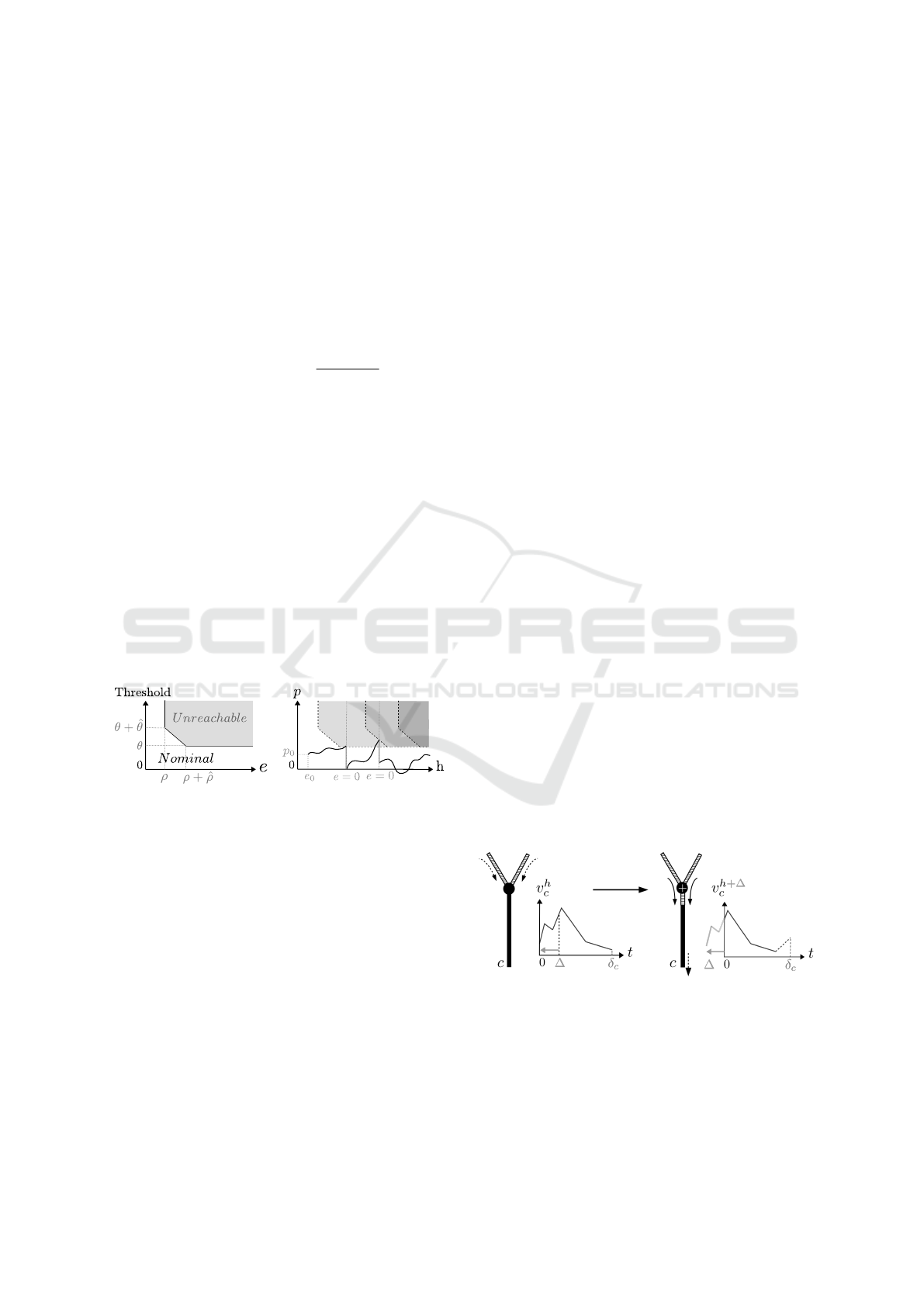
Figure 6: State of a compartment and ∆-shift (Deﬁnition 9).

Deﬁnition 9. [∆-shift] Given a neuron N and an in-

put signal S = {ω

}

s∈Sy(N)

, let V

= {v

}

c∈Co(N)

be a dendritic state of N at time h and let ∆ ∈ IR

such that 0 6 ∆ 6 in f ({δ

| c ∈ CCo(c)}). For any

compartment c ∈ Co(N), the ∆-shift of v

(noted ∆-

shift(v

,S )), is the function v : [0,δ

] → IR such that:

BIOINFORMATICS 2018 - 9th International Conference on Bioinformatics Models, Methods and Algorithms

• ∀t ∈ [0, δ

−∆], v(t) = v

(t + ∆);

• ∀t ∈ [δ

−∆, δ

], v(t) = (

∑

∈CCo(c)

(t −δ

+∆) +

∑

s∈CSy(c)

(h +t −δ

+ ∆)) ×α

By extension, the family composed of the ∆-shifts of

all the v

∈V is called the ∆-shift of V according to

S and it is noted ∆-shift(V, S ).

Theorem 1. [Compartments dynamics] Given an

initial dendritic state V

of a neuron N and an input

signal S = {ω

}

s∈Sy(N)

. There exists a unique den-

dritic state family {V

}

h∈IR

such that:

• V

= V

;

• for any ∆ such that 0 6 ∆ 6 in f ({δ

|c ∈Co(N) ∧

> 0}) and for any h, V

h+∆

=∆-shift(V

,S ).

Deﬁnition 10. [Dynamics of a neuron] Given a neu-

ron N, a state η

= (V

, p

) and an input signal

S = {ω

}

s∈Sy(N)

, the dynamics of N, according to S

with η

as initial state, is the function d

: IR

→ ζ

deﬁned by:

• d

(0) = η

• ∀h ∈IR

, d

(h) = η

= (V

, p

) where:

– V

is deﬁned as in Theorem 1;

– Consider beforehand the lipschitzian function

F(u) =

∑

c∈In(∇)

(0). According to Technical

lemma 1, there exists a unique function P

such

that P

, p

,0) = p

and ∀u,

,u)

F(u) −γ.P

, p

,u). If P

, p

,u) is con-

tinuous on the interval ]0,h], then e = e

+ h.

Otherwise, let u

be the greatest u such that

, p

,u) is discontinuous, then e = h −u

– Considering the previous P

function, p =

, p

,h).

4 SIMULATION OF THE HYBRID

MODEL AND MODEL

CHECKING

Our goal is to use our framework to prove particu-

lar properties of neurons. Our framework deﬁnes a

hybrid process of signal integration via the dendritic

tree, preserving linear equations. However, the inte-

gration at the soma inevitably induces a differential

equation in order to preserve the essence of the bio-

logical functioning. This is unfortunately detrimental

to computer-aided formal proving approaches. There-

fore, the following step was to discretize time. Obvi-

ously, the smaller the time step is and the more ac-

curate the result will be. But, one must also consider

the computational cost. The proper trade-off largely

depends on the system we are interested in. When

considering neuron spiking, events are usually as-

sumed to be synchronous when happening in a given

1 to 5 milliseconds time window (Izhikevich, 2006;

Brette, 2012; Gr

un et al., 1999). Therefore, our time

step should be less than 1 millisecond. According

to (Bower, 2003), 0.01 millisecond is an appropriate

choice when looking at the shape of the action poten-

tial. Here, as we consider discrete spikes, we have

chosen 0.1 millisecond as a reasonable time step (∆t).

4.1 Timing Discretization

For simulation and model checking purposes, all the

temporal parameters have to be expressed in multiples

of ∆t.

Synapses. Usually,

τ (sometimes called time-to-

peak) goes from one to tens of milliseconds and

τ is

most of the time greater (Williams and Stuart, 2002;

Magee and Cook, 2000). This makes our time step ap-

propriate, as a sufﬁciently large number of points will

be considered in the trace of the signal (Figure 7).

Figure 7: Simulation of a trace (v

s,ω

) of an input signal (ω)

on a synapse (s) with arbitrary parameters (ν = 3,

τ = 6

and

τ = 12). It is encoded in Lustre and simulated with

luciole. On the top is represented a trace in response to

a single spike. On the bottom, the trace exhibits temporal

summation.

Compartments. The delay for crossing a compart-

ment (δ) being expressed in multiples of ∆t, com-

partments smaller than 1∆t will be considered as

null. This assumption may lead to kind of clusters of

synapses, which are observed experimentally (Stuart

et al., 2016; G

okc¸e et al., 2016).

Figure 8: Division of a compartment into sub-

compartments for proper discretization.

For each compartment, we deﬁne n = δ/∆t sub-

compartments (noted subC, see Figure 8). Sub-

compartments parameters are deﬁned as follows:

Computer-aided Formal Proofs about Dendritic Integration within a Neuron

subC

= 1∆t and α

subC

√

α (where n is the num-

ber of sub-compartments in the original compartment

and α is the attenuation of the original compartment).

Given this representation, the dynamics is done by

shifting all the sub-compartments at a time.

Soma. The major motivation for discretization is the

time discretization at the soma. Basically, we chose

to replace a differential equation with a difference

to be solved at discrete time intervals (∆t). From

Lemma 1, we have:

= F(t) −γ.P(t). Once time is

discretized, since P is piecewise linear, this equation

is equivalent to

P(t+∆t)−P(t)

∆t

= F(t) −γ.P(t). We thus

have P(t +∆t)−P(t) = (F(t)−γ.P(t)).∆t. Therefore,

we should use the following equation:

P(t + ∆t) = F(t).∆t + P(t).(1 −γ.∆t).

Linearity properties (resulting from Deﬁnition 3)

make this discretization exact. However, spikes times

are approximated and this could lead to some error

accumulation. Nevertheless, there is a limited risk

of missing any spikes as the ARP is in the order

of a millisecond, largely limiting the maximal fre-

quency (Johnson, 2003).

4.2 Formal Proofs using Model

Checking: a Simple Example

Based on our discretized model, we can use model

checking in order to prove properties on neurons with

dendrites in a computer-aided manner. Model check-

ing allows one to automatically verify if a model sat-

isﬁes a given property. We have chosen to encode our

model in Lustre and using Kind2 as model checker

(with z3 solver).

Lustre. Lustre is a synchronous programming lan-

guage, working with ﬂows. It beneﬁts from a formal

deﬁnition and it is particularly suited to reactive sys-

tems. A program in Lustre consists of nodes. A node

computes outputs based on algebraic equations, ac-

counting for input variables. All variables are typed.

Local variables can be declared using the keyword

var. The body of the node is composed of set of

equations always true, surrounded by the keywords

let and tel. For this reason, Lustre is a declarative

language and not imperative. A node is declared as

follows:

node nameOftheNode(input1: typeInput1; ...)

returns(output1: typeOutput1; ...);

var localVar1: typeVar1; ...;

let

Equations;

tel

In Lustre, a variable does not carry a given value

but a function of time, that is an inﬁnite sequence of

values. As an example, to deﬁne a variable x, we

should use the following syntax:

x = initial value -> induction principle;

The values carried by a variable are computed by

a temporal recurrence expression which can depend

on other variables. The initial value is the ﬁrst

value of the inﬁnite sequence. It splits up the other

values by the operator -->. Lustre has some elemen-

tary basic types (bool, int, real) and usual operators

can be used on them ( +,-,*, etc.; and,or,not;

if then else). As an example, if a variable x is the

inﬁnite ﬂow (x

, x

,...) and another variable y is the

inﬁnite ﬂow (y

, y

,...) then, the variable z = x + y is

the inﬁnite ﬂow (z

= x

+ y

, z

= x

+ y

,...).

Moreover there exists in Lustre an additional op-

erator to deal with logical time: pre(). It acts as a

memory by providing access to the previous value of

a variable at a given time. For instance if the variable

x is deﬁned by x = 0 -> pre(x)+1, the ﬂow will be

equal to 0 at time 0, equal to 0+1 = 1 at time 1, equal

to 1 + 1 = 2 at time 2, and so on.

Any node can be simulated by a dedicated Lustre sim-

ulator called luciole (see Figure 7).

Kind2. There are several model checkers for Lus-

tre. Kind2 relies on SMT (Satisﬁabitily Modulo The-

ories) based k-induction and it proved to be efﬁcient

contrary to others model checkers such as lesar, nbac,

luke and rantanplan (De Maria et al., 2016).

Kind2 is able to prove mathematical properties en-

coded as Lustre node: We write, in Lustre, the prop-

erty as a boolean variable and Kind2 veriﬁes if it is

always true. As an example, to check if a variable x

is equal to a variable y, meaning that at each time step

the values of the two variables are the same, one can

write the following node:

node property(x, y : int) returns (proof: bool);

let

proof = x = y;

tel

Here, the output of the node property returns the

value of proof which is true when x = y and false

otherwise. The property is thus satisﬁed if proof is

always true whatever the values of x and y, at any time

step.

A Simple Example.

As a ﬁrst property to check, we have decided to

compare the outputs of simple neurons for a given in-

put and given initial states.

Let us consider the two neurons illustrated in Fig-

ure 9. Following Deﬁnition 10 and since both neu-

rons have the same soma parameters, it is sufﬁcient

to compare the output of their dendritic forests. We

have thus ignored the soma at ﬁrst. We have en-

coded synapses and compartments in Lustre by deﬁn-

BIOINFORMATICS 2018 - 9th International Conference on Bioinformatics Models, Methods and Algorithms

Figure 9: Example of two simple neurons. Their parameters

are δ = 1 and α = 0.5 for all black compartments (in neuron

), δ = 2 and α = 0.25 for the light grey compartment (c

in neuron N

), δ = 3 and α = 0.125 for dark gray compart-

ments (c

and c

in neuron N

). Synapses s

are deﬁned

by ν = 5,

τ = 5,

τ = 15, synapses s

are deﬁned by ν = 3,

τ = 6,

τ = 12 and synapses s

are deﬁned by ν = −5,

τ = 5,

τ = 10. N

and N

both have the same soma parameters.

ing nodes for each of them. Below, we show as

an example, how a compartment can be deﬁned for

δ = 3.∆t (with α = 0.125). Compartments with dif-

ferent parameters are encoded in the same way.

node comp3dt (I, init1, init2, initO : real)

returns (O : real);

var c1, c2, alphaSubC : real;

let

alphaSubC = 0.5;

c1 = init1 -> pre(I) * alphaSubC;

c2 = init2 -> pre(c1) * alphaSubC;

O = initO -> pre(c2) * alphaSubC;

tel

As shown in Figure 8, the compartment is divided into

3 sub-compartments with δ

subC

= 1.∆t and α

subC

√

0.125 = 0.5. The node comp3dt takes as inputs

real variables: the input (I) of the compartment

(representing the signals coming from the contribu-

tor compartments or synapses) and the initial states

(init1, init2, initO) of each sub-compartment.

It then computes the output (O) of the whole com-

partment (with initO as initial value). The variables

(c1) and (c2) are the outputs of respectively the ﬁrst

and the second sub-compartments. The output of the

ﬁrst sub-compartment is computed from the value of

the input I, one ∆t before (using the operator pre()).

Similarly, the output of the second sub-compartment

is computed from the output of the ﬁrst one, and so

on.

To encode synapses, one node is required for each

couple of parameters (

τ,

τ). The node presented below

encodes a simple excitatory synapse with ν = 1,

τ = 2

and

τ = 4.

node synapseE2_4 (omega : bool)

returns (vs : real);

var nu, hatTau, checkTau : real;

o1, o2, o3, o4, o5 : bool;

let

nu = 1.0;

hatTau = 2.0;

checkTau = 4.0;

o1 = false -> pre(omega);

o2 = false -> pre(o1);

o3 = false -> pre(o2);

o4 = false -> pre(o3);

o5 = false -> pre(o4);

vs = 0.0 -> (if o1

then nu/hatTau

else 0.0)

+ (if o2

then 2.0*nu/hatTau

else 0.0)

+ (if o3

then nu-nu/checkTau

else 0.0)

+ (if o4

then nu-2.0*nu/checkTau

else 0.0)

+ (if o5

then nu-3.0*nu/checkTau

else 0.0);

tel

The node synapseE2_4 takes as input the boolean

variable omega that represents the spikes sequence

and computes the output vs that is the trace of the

input signal omega on the synapse. The local vari-

ables nu, hatTau and checkTau are respectively the

maximal potential variation triggered by a spike, the

rise time and the descent delay. As shown in Fig-

ure 3, the contribution of a spike to the trace at a

given time greatly depends on the time elapsed since

the spike occurrence. The local boolean variable o1

is true if omega was true one time step before the cur-

rent time, meaning that there was a spike at the pre-

vious time. Similarly, o2 is true if omega was true

two time steps before the current time, meaning that

there was a spike two times before, and so on. In

this case, we have to look up to

τ +

τ −1 = 5 time

steps back because beyond this time window a spike

no longer inﬂuences the trace. In order to produce a

temporal summation, the trace is computed from the

contributions of all the preceding spikes. In the same

way, we deﬁne nodes for inhibitory synapses called

synapseIx_y where nu is a negative real number.

Once synapses and compartments are encoded as

Lustre nodes, it is possible to deﬁne the entire den-

dritic forest for both neurons:

node neuron1(I1, I2, I3 : bool)

returns (O : real);

var S1, S2, S3, C1, C2, C3, C23,

initC1, initC2, initC3, initC23,

initO : real;

let

initC1 = 0.0; initC2 = 0.0;

initC3 = 0.0; initC23 = 0.0;

initO = 0.0;

S1 = synapseE5_15(I1);

S2 = synapseE6_12(I2);

Computer-aided Formal Proofs about Dendritic Integration within a Neuron

S3 = synapseI5_10(I3);

C1 = comp1dt(S1, initC1);

C2 = comp1dt(S2, initC2);

C3 = comp1dt(S3, initC3);

C23 = comp1dt(C2 + C3, initC23);

O = comp1dt(C1 + C23, initO);

tel

node neuron2(I1, I2, I3 : bool)

returns (O : real);

var S1, S2, S3, C1, C2, C3,

initC11, initC12, initC21, initC22,

initC23, initC31, initC32, initC33,

initO : real;

let

initC11 = 0.0; initC12 = 0.0;

initC21 = 0.0; initC22 = 0.0;

initC23 = 0.0; initC31 = 0.0;

initC32 = 0.0; initC33 = 0.0;

initO = 0.0;

S1 = synapseE5_15(I1);

S2 = synapseE6_12(I2);

S3 = synapseI5_10(I3);

C1 = comp2dt(S1,initC11,initC12);

C2 = comp3dt(S2,initC21,initC22,initC23);

C3 = comp3dt(S3,initC31,initC32,initC33);

O = initO -> C1 + C2 + C3;

tel

Both nodes (neuron1 and neuron2) compute a

boolean output (O) from boolean inputs I1, I2, I3

(representing sequences of spikes at synapses). As

mentioned before, the two neurons have the same

set of synapses (Figure 9). The real variables

S1, S2, S3 are the outputs of the nodes encoding

respectively synapses s

, s

with I1, I2, I3 as

inputs. They are thus used as inputs for compart-

ments comp1dt, comp2dt, comp3dt whose outputs

C1, C2, C3, C23 are, in turn, used as inputs for

other compartments. It allows ultimately to compute

the output of the whole dendritic forest. For the sake

of simplicity, compartment initial states were ﬁxed to

zero in both neurons. Under this condition and by

considering constant inputs (always equal to true or

false), we have proven that these two particular neu-

rons (Figure 9) always produce the same outputs. All

the possible inputs combinations (2

= 8) were veri-

ﬁed. Below is the Lustre node encoding the property

with I1 and I2 being always true and I3 being always

false:

node equivalence(gost : bool, epsilon: real)

returns (proof: bool);

var I1, I2, I3 : bool;

let

I1 = true;

I2 = true;

I3 = false;

proof = abs(neuron1(I1, I2, I3)

- neuron2(I1, I2, I3)) < epsilon;

tel

Because neurons compute with real numbers,

rounding errors in computation prevent to deﬁne

proof as the simpler equality neuron1(I1, I2,

I3) = neuron2(I1, I2, I3);. In fact, with our

example, this equality version the proof succeeds too:

neuron1 and neuron2 make the same approxima-

tions.

We have also proven that the property is satis-

ﬁed for other arbitrary inputs. As an example, we

used I1 being true on 1 time step in 50, I2 be-

ing true on 1 time step in 10 and I3 being true on

1 time step in 20.

For constant inputs, the model checker is remark-

ably efﬁcient. For inputs with frequencies, we reach

the limits of kind2 on a standard laptop, as the proof

takes several hours.

Here, proofs have been entirely automatically han-

dled by the model checker. Even though this example

is simple, the ability of Kind2 to fully perform proofs

without human guidance is encouraging.

5 CONCLUSION

We deﬁned here the ﬁrst hybrid formal model of neu-

ron taking into account the morphology and its key

role in neuronal computation. Our aim was to use for-

mal methods from computer science to prove proper-

ties based on this framework. In order to make au-

tomatic proofs, we have used model checking. The

main interest of this proof-based approach is the ex-

ploration of the whole space of possibilities inside a

single proof. However, it requires models with dis-

crete time. We thus proposed relevant abstractions of

the neuron structure and dynamics with a subsequent

time discretization.

Nevertheless, the number of parameters is still

huge and it increases as we get closer to the biolog-

ical reality. A “standard” neuron has thousands of

synapses located on its dendrites making the system

very complex.

Here, we successfully used model checking on a

simple example. We proved that two particular neu-

rons with different dendritic structures can have the

same input/output function. This ﬁrst result empha-

sises the crucial role of delays and attenuations rather

than the importance of the precise dendrites morphol-

ogy. It is partly a consequence of the hypotheses and

choices we made. If we would like to incorporate

some other biological properties (such as shunting)

to our model, it would probably change this basic re-

sult (H

ausser and Mel, 2003; Paulus and Rothwell,

2016; Gorski et al., 2017). But, even though our

modelling relies on several simplifying assumptions,

BIOINFORMATICS 2018 - 9th International Conference on Bioinformatics Models, Methods and Algorithms

it constitutes a ﬁrst track to investigate the impact of

the morphology on the neuron function, the ﬁrst for-

mal one.

As a direct continuation of this work, it would be

interesting to make more general proofs and possi-

bly with more complex and biologically relevant ex-

amples. The ultimate aim would be to automatically

ﬁnd constraints on parameters, such as observed de-

lays provided by dendrites, for a model to satisfy a

given behaviour. In another research direction, we

think about building neuronal circuits. This would

probably bring insights on how the neuronal structure

could enable the emergence of complex behaviour at

a larger scale.

REFERENCES

Bianchi, S., Stimpson, C. D., Bauernfeind, A. L., Schapiro,

S. J., Baze, W. B., McArthur, M. J., Bronson, E.,

Hopkins, W. D., Semendeferi, K., Jacobs, B., et al.

(2012). Dendritic morphology of pyramidal neu-

rons in the chimpanzee neocortex: regional special-

izations and comparison to humans. Cerebral cortex,

23(10):2429–2436.

orgers, C. (2017). Quadratic integrate-and-ﬁre (qif) and

theta neurons. In An Introduction to Modeling Neu-

ronal Dynamics, pages 51–55. Springer.

Bower, J.M., B. D. (2003). The book of GENESIS: explor-

ing realistic neural models with the General Neural

Simulation System. Internet Edition.

Brette, R. (2003). Mod

eles impulsionnels de r

eseaux de

neurones biologiques. PhD thesis, Universit

e Pierre et

Marie Curie-Paris VI.

Brette, R. (2012). Computing with neural synchrony. PLoS

computational biology, 8(6):e1002561.

Brette, R. and Gerstner, W. (2005). Adaptive exponen-

tial integrate-and-ﬁre model as an effective descrip-

tion of neuronal activity. Journal of neurophysiology,

94(5):3637–3642.

Brunel, N. and Van Rossum, M. C. (2007). Lapicques 1907

paper: from frogs to integrate-and-ﬁre. Biological cy-

bernetics, 97(5-6):337–339.

Cook, E. P. and Johnston, D. (1997). Active dendrites re-

duce location-dependent variability of synaptic input

trains. Journal of neurophysiology, 78(4):2116–2128.

De Maria, E., Muzy, A., Gaff

e, D., Ressouche, A., and

Grammont, F. (2016). Veriﬁcation of temporal prop-

erties of neuronal archetypes modeled as synchronous

reactive systems. In International Workshop on Hy-

brid Systems Biology, pages 97–112. Springer.

okc¸e, O., Bonhoeffer, T., and Scheuss, V. (2016). Clusters

of synaptic inputs on dendrites of layer 5 pyramidal

cells in mouse visual cortex. eLife, 5:e09222.

Gorski, T., Veltz, R., Galtier, M., Fragnaud, H., Telenczuk,

B., and Destexhe, A. (2017). Inverse correlation pro-

cessing by neurons with active dendrites. bioRxiv.

un, S., Diesmann, M., Grammont, F., Riehle, A., and

Aertsen, A. (1999). Detecting unitary events without

discretization of time. Journal of neuroscience meth-

ods, 94(1):67–79.

ausser, M. and Mel, B. (2003). Dendrites: bug or feature?

Current opinion in neurobiology, 13(3):372–383.

ausser, M., Spruston, N., and Stuart, G. J. (2000). Di-

versity and dynamics of dendritic signaling. Science,

290(5492):739–744.

Hodgkin, A. L. and Huxley, A. F. (1952). A quantitative

description of membrane current and its application to

conduction and excitation in nerve. The Journal of

physiology, 117(4):500–544.

Hu, H. and Vervaeke, K. (2017). Synaptic integration in

cortical inhibitory neuron dendrites. Neuroscience.

Izhikevich, E. M. (2006). Polychronization: computation

with spikes. Neural computation, 18(2):245–282.

Johnson, L. R. (2003). Essential medical physiology. Aca-

demic Press.

Johnston, D. and Narayanan, R. (2008). Active dendrites:

colorful wings of the mysterious butterﬂies. Trends in

neurosciences, 31(6):309–316.

Koch, C. (2004). Biophysics of computation: information

processing in single neurons. Oxford university press.

Lapicque, L. (1907). Recherches quatitatives sur

l’excitation electrique des nerfs traitee comme polari-

sation. J. Physiol. Pathol. Gen., 9:620–635.

Maass, W. (1996). Lower bounds for the computational

power of networks of spiking neurons. Neural com-

putation, 8(1):1–40.

Maass, W. (1999). Computing with spiking neurons. Pulsed

neural networks, 85.

Magee, J. C. and Cook, E. P. (2000). Somatic epsp am-

plitude is independent of synapse location in hip-

pocampal pyramidal neurons. Nature neuroscience,

3(9):895.

Manita, S., Miyakawa, H., Kitamura, K., and Murayama,

M. (2017). Dendritic spikes in sensory perception.

Frontiers in cellular neuroscience, 11.

McCulloch, W. S. and Pitts, W. (1943). A logical calculus

of the ideas immanent in nervous activity. The bulletin

of mathematical biophysics, 5(4):115–133.

Mel, B. W. (1994). Information processing in dendritic

trees. Neural computation, 6(6):1031–1085.

Mohan, H., Verhoog, M. B., Doreswamy, K. K., Eyal,

G., Aardse, R., Lodder, B. N., Goriounova, N. A.,

Asamoah, B., B. Brakspear, A. C., Groot, C., et al.

(2015). Dendritic and axonal architecture of individ-

ual pyramidal neurons across layers of adult human

neocortex. Cerebral Cortex, 25(12):4839–4853.

Paulus, W. and Rothwell, J. C. (2016). Membrane resis-

tance and shunting inhibition: where biophysics meets

state-dependent human neurophysiology. The Journal

of physiology, 594(10):2719–2728.

Popper, K. R. (1963). Conjectures and refutations: the

growth of scientiﬁc knowledge.

Rall, W. (1959). Branching dendritic trees and motoneu-

ron membrane resistivity. Experimental neurology,

1(5):491–527.

Computer-aided Formal Proofs about Dendritic Integration within a Neuron

Rall, W. (1962). Theory of physiological properties of den-

drites. Annals of the New York Academy of Sciences,

96(1):1071–1092.

Rall, W. (1967). Distinguishing theoretical synaptic poten-

tials computed for different soma-dendritic distribu-

tions of synaptic input. Journal of neurophysiology,

30(5):1138–1168.

Rall, W. (2011). Core conductor theory and cable properties

of neurons. Comprehensive physiology.

Remme, M. W., Lengyel, M., and Gutkin, B. S. (2010).

Democracy-independence trade-off in oscillating den-

drites and its implications for grid cells. Neuron,

66(3):429–437.

Stuart, G., Spruston, N., and H

ausser, M. (2016). Dendrites.

Oxford University Press.

Stuart, G. J. and Spruston, N. (2015). Dendritic integra-

tion: 60 years of progress. Nature neuroscience,

18(12):1713–1721.

Sun, Q., Srinivas, K. V., Sotayo, A., and Siegelbaum, S. A.

(2014). Dendritic na+ spikes enable cortical input to

drive action potential output from hippocampal ca2

pyramidal neurons. Elife, 3:e04551.

Williams, S. R. and Stuart, G. J. (2002). Dependence of

epsp efﬁcacy on synapse location in neocortical pyra-

midal neurons. Science, 295(5561):1907–1910.

BIOINFORMATICS 2018 - 9th International Conference on Bioinformatics Models, Methods and Algorithms