
Mining Sequential Patterns for Appliance Usage Prediction
Mathieu Kalksma
1
, Brian Setz
2
, Azkario Rizky Pratama
2
, Ilche Georgievski
3
and Marco Aiello
2
1
Quintor B.V., Ubbo Emmiussingel 112, 9711 BK Groningen, The Netherlands
2
Distributed Systems, Johann Bernoulli Insititute, University of Groningen,
Nijenborgh 9, 9747 AG, Groningen, The Netherlands
3
Sustainable Buildings, Nijenborgh 9, 9747 AG, Groningen, The Netherlands
Keywords:
Appliance Usage Prediction, Energy Consumption Prediction, Sequential Pattern Mining.
Abstract:
Reducing the energy consumption in buildings can be achieved by predicting how energy-consuming appli-
ances are used, and by discovering their usage patterns. To mine patterns, a smart-metering architecture needs
to be in place complemented by appropriate data analysis mechanisms. These usage patterns can be employed
to optimize the way energy from renewable installations, home batteries, and even microgrids is managed.
We present an approach and related experiments for mining sequential patterns in appliance usage. We mine
patterns that allow us to perform device usage prediction, energy usage prediction, and device usage predic-
tion with failed sensors. The focus of this work is on the sequential relationships between the state of distinct
devices. We use data sets from three distinct buildings. The data is used to train our modified Support-Pruned
Markov Models which use a relative support threshold. Our experiments show the viability of the approach,
as we achieve an overall accuracy of 87% in device usage predictions, and up to 99% accuracy for devices that
have the strongest sequential relationships. For these devices, the energy usage predictions have an accuracy
of around 90%. Predicting device usage with failed sensors is feasible, assuming there is a strong sequential
relationship for the devices.
1 INTRODUCTION
Electric appliances are responsible for a significant
portion of a household’s energy consumption, hav-
ing a strong impact on a household’s carbon foot-
print. In fact, according to the U.S Energy Infor-
mation Administration (EIA), the energy consump-
tion for household appliances, electronics and light-
ing is responsible for 37% of the total energy con-
sumed by households in 2016 (EIA, 2016). This is an
increase of 10% compared to 1993. Since household
appliances and other electronics are responsible for an
ever-increasing share of a household’s consumption,
it is important to focus on energy usage optimization
efforts in order to meet global greenhouse gases emis-
sion goals.
Smart-metering architectures are essential to gain
insight into the way energy is used and to predict the
future energy consumption. These predictions enable
the optimization of energy production and manage-
ment by smart scheduling of renewable resources and
devices. At the consumer end of the spectrum, this
means measuring and monitoring the way appliances
are utilized and predicting their future usage patterns.
With the emergence of the Internet of Things, we ex-
pect an increasing number of appliances to be con-
nected to the Internet. These appliances shall be able
to provide real-time information on their energy us-
age as a service. Till then, we can use commercially
available electric plug monitoring devices to collect
consumption information. The collected information
can then be exploited to make predictions about future
device utilization and energy consumption. For exam-
ple, in previous work, we investigated device recog-
nition by means of an aggregated power consumption
observed at a single point measurement (Pratama et
al., In Press). This type of information is essential
for home and building energy management systems,
and also has potential for use in smart and micro-grid
applications.
In this work, we focus on mining patterns from
household appliances and propose an approach based
on high-order Markov models to predict: 1) the us-
age of devices, 2) the expected energy footprint, and
3) the usage of a device with a failed sensor. We
focus specifically on the sequence of device states
over time, and the patterns that exist there. The
model we propose is based on a modified version of
Kalksma, M., Setz, B., Rizky Pratama, A., Georgievski, I. and Aiello, M.
Mining Sequential Patterns for Appliance Usage Prediction.
DOI: 10.5220/0006669500230033
In Proceedings of the 7th International Conference on Smart Cities and Green ICT Systems (SMARTGREENS 2018), pages 23-33
ISBN: 978-989-758-292-9
Copyright
c
2019 by SCITEPRESS – Science and Technology Publications, Lda. All rights reserved
23

the Support-Pruned Markov Model (Deshpande and
Karypis, 2004) that utilizes a relative support thresh-
old. The results of our experiments demonstrate the
viability of the approach, especially for device usage
predictions. To verify the validity of the model and
the prediction algorithms, we consider three distinct
datasets coming from real-world installations. Two
data sets are from actual households, and one data set
is from an office building functioning as a living lab.
We use these data sets to train our model and to eval-
uate the quality of the predictions.
The remainder of the paper is organized as fol-
lows. In Section II, we provide a formal definition of
the proposed model and describe the algorithms be-
hind our designed solution. Section III describes the
experimentation on three distinct data sets. Section IV
presents related work, while concluding remarks are
presented in Section V.
2 APPROACH AND PROPOSAL
We aim to discover sequential patterns in the state
changes of devices over time, in order to forecast the
future state changes and energy footprint. A Markov
Model (MM) enables the prediction of future states
based on the current state. In MM terms, the current
state refers to the current state of the set of devices.
The future state represents the predicted state changes
for a set of devices, given the current state.
A high-order MM considers more historical ac-
tions to predict the future state. In other words, the
k
th
-order MM considers the sequence of the previous
k states when predicting the next state. The All-K
th
-
Order Markov model (Pitkow and Pirolli, 1999) ad-
dresses the issue of reduced coverage by looking for a
sequence in the k
th
-order and, if not found, it contin-
ues searching the lower orders. The disadvantage of
All-K
th
-Order Markov models is that the state space
expands drastically, as all models from 1 to k have to
be trained and stored.
The Support-Pruned Markov Model (SPMM) is
based on the All-K
th
-Order Markov model (Desh-
pande and Karypis, 2004). It introduces the concept
of pruning in order to reduce the large state space of
All-K
th
-Order models. The state pruning relies on the
observation that a state with low support often has
a low prediction accuracy associated with it. Prun-
ing these states increases the overall accuracy and
reduces the state-space complexity. States with low
support are identified by applying an absolute fre-
quency threshold, φ. The frequency threshold is the
minimum absolute number of instances in the train-
ing set required for a state to be included in the model.
If there are less than φ instances, the support for the
state is too low and it is pruned. As higher-order states
often have less support in the training set, these are
more likely to be removed, dramatically decreasing
the state-space complexity.
2.1 Model Definition
We propose an adapted version of the SPMM in
which, instead of an absolute frequency threshold φ, a
relative support threshold r is applied, inspired by the
method described in (Agrawal et al., 1993). Using
a relative threshold, we ensure that we do not prune
subsequences with a strong relationship. We employ
the following definitions:
Devices: Let V = {v
1
,...,v
n
} be a set of de-
vices. At any given time t, a device has a binary
state s, where s = 1 and s = 0 are equivalent to the
device being turned on or off, respectively. The his-
torical data of a device v
i
is defined as a set S
v
i
=
{< t
1
,s
1
>,...,< t
m
,s
m
>}, where s
1
,...,s
m
are the
historical states and t
1
,...,t
m
are their corresponding
timestamps.
Transaction: A transaction τ is defined as a set of
devices for which s = 1 at a given time t, thus τ(t) =
{v
i
|∀i : S
v
i
(t) = 1}. A set of transactions T is an or-
dered set of transactions such that ∀i, j : i < j,T
i
< T
j
;
all transactions in the set T are ordered by time in as-
cending order.
Sequence: Given a set of transactions T , a se-
quence seq is defined as the transitions in time be-
tween the transactions τ ∈ T . The maximum times-
pan between the first element in T and the last ele-
ment (T
0
− T
|T |
) is referred to as m. In this work, m is
always denoted in minutes. To further reduce the state
space, next to the relative support threshold, a maxi-
mum length of a sequence is enforced. Let |seq| ≤ k,
where k is the maximum length of a sequence.
For example, consider the set of devices to be
V = {A,B,C}, τ
1
= {A}, τ
2
= {B,C} and τ
3
= {A},
and τ
1
transits to B and C via τ
2
and to A via τ
3
.
Thus, according to our definitions, the transaction
set T = {τ
1
,τ
2
,τ
3
} encompasses all of the following
sequences: {ABA},{ACA},{AB}, {AC},{A},{B},
{C}, {AA}, {BA} and {CA}.
Support: The relative support of a sequence seq
i
is defined as supp(seq
i
) = w(seq
i
)/w(seq
p
i
), where w
is a function returning the number of times a sequence
occurs in the transaction set T and seq
p
i
is the par-
ent sequence of seq
i
. For example, given a sequence
{A,B,C}, the parent sequence is {A,B}. A sequence
is supported if, and only if, the support for that se-
quence is above r, the minimal support threshold. We
use a relative support threshold instead of an absolute
SMARTGREENS 2018 - 7th International Conference on Smart Cities and Green ICT Systems
24

support threshold to prevent the pruning of sequences
that have a low initial support but a strong relationship
with its child sequences.
To illustrate the difference between absolute and
relative thresholds, let there be three sequences:
seq
0
= {A}, seq
1
= {AB}, and seq
2
= {ABC}. We as-
sume the following number of occurrences after 100
measurements: seq
0
occurs a 100 times, seq
1
occurs
10 times, and seq
2
occurs 9 times. We set the thresh-
old to be r = 0.1. The absolute support for seq
2
is 0.09
(r = 9/100), whereas the relative support supp(seq
2
)
equals 0.9 (r = 90/100) as seq
2
follows seq
1
90%
of the time. If the absolute support were used, seq
2
would have been pruned (0.09 < 0.1) despite having
a very strong relationship with seq
1
. Thus, we choose
to use the relative support to prevent the pruning of
strong relationships between (sub)sequences.
2.2 Predictive Algorithms
We utilize algorithms to solve the problems of device
state prediction, energy consumption prediction, and
device state prediction with a failed sensor. We de-
scribe each of the algorithms in the following sub-
sections, while a complete definition of the pseudo-
code for each individual algorithm can be found
in (Kalksma, 2016).
2.2.1 Device State Prediction
The device state prediction is a prediction of which
devices will be used in the next m time units. To pre-
dict the state of devices in the next m time units, we
take a stream of real-time transactions and store the
last x transactions, such that the time span between
T
0
and T
x
is less than m time units. All possible se-
quences are determined based on the cached transac-
tions. When the model is trained, it predicts which
devices will be in the “on” state for the next m time
units.
Figure 1: Illustration of a transactions time line.
Figure 1 provides an example of a time line with
m = 3 time units. The transactions that occurred at
t − 0, t − 1 and t − 2 have been cached. At t − 0 de-
vice A is in the on state (s
i
= 1), at t −1 device C is on,
and at t − 2 both device A and B are on. In this case,
the possible sequences based on the cached trans-
actions are {ACA}, {AC}, {A},{BCA},{BC},{B},
{AA},{BA},{CA} and {C}.
For each device a certainty P is determined,
which is the probability for a device to be in use given
a certain supported sequence. The certainty P can be
defined in two ways: average certainty and weighted
average certainty. The average certainty, P
avg
, is the
sum of all probabilities of the supported sequences,
divided by the total number of supported sequences.
The weighted average certainty, P
wavg
, is the sum of
all probabilities of the supported sequences times a
weight w, divided by the number of supported se-
quences. The methods used to calculate P
avg
and
P
wavg
are referred to as avg and wavg, respectively.
If P is greater than 0.5, the device is considered to be
used (s = 1) in the next m time units.
2.2.2 Energy Consumption Prediction
Next, we predict the energy consumption, also re-
ferred to as the energy footprint, of a set of devices.
The prediction of energy consumption is based on an
extension of the state prediction algorithm. The out-
put of the state prediction is used as input for the en-
ergy consumption prediction. When a device is pre-
dicted to be in use for a given time interval, we pre-
dict the energy consumption for this interval. In or-
der to perform these predictions, a second Support-
Pruned Markov Model is trained. The model predicts
the transitions between the energy consumption lev-
els of a device. The energy consumption levels for
each device are defined in bands. For example, an
energy consumption band could be {0W , 5W , 10W ,
30W }, where 0, 5, 10, and 30 are the levels we iden-
tified for this specific device. The actual consumption
measurements are rounded to the nearest band. From
these measurements, a Markov chain is created based
on the energy consumption measurements of the last
m = 3 time units.
To predict the future energy consumption of a
device, we follow a similar approach to training as
we did for the energy consumption model. First,
the observed energy consumption measurements are
rounded to the nearest band and a sequence is cre-
ated from the last three measurements. When the state
prediction indicates that a device will be used, the en-
ergy consumption model is used to retrieve the pre-
dicted energy consumption for the given device. Us-
ing the current consumption sequence as input, the
model predicts the future energy consumption by se-
lecting the most probable sequence. When the input
sequence is not available in the model, the algorithm
will select the last known consumption as the pre-
dicted energy consumption. If the state prediction al-
Mining Sequential Patterns for Appliance Usage Prediction
25

Table 1: Properties of the data sets used in the evaluation.
Properties Data sets
Name RUG ECO1 ECO2
Number of devices 5 4 7
Measurement Period 195 days 237 days 245 days
Coverage (
N
records
N
minutes
) 77.84% 99.64% 98.58%
Training set (N
records
) 131,386 211,619 175,679
Validation set (N
records
) 86,066 120,960 169,860
gorithm concludes that the device will not be used, the
lowest consumption band is selected as the predicted
energy consumption.
For example, given a device with bands defined
as {0W , 5W , 10W , 30W }, and an actual consumption
history of {1.2W , 4.3W , 12W , 19W }. The histori-
cal consumption will be rounded to the nearest band,
resulting in the following measurements: {0W , 5W ,
10W , 10W }. The first three measurements (m = 3)
of the consumptions for this device are 0W , 5W and
10W . Thus, the state sequence 0 − 5 − 10 is trained
with a future state of 10W . Once the model is trained
on a data set, it enables the prediction of the most
likely energy consumption for the next time interval
for each sequence per device.
2.2.3 Device State Prediction with Failed Sensor
Finally, we predict the state of devices while one of
the sensors has failed. The algorithm for this pre-
diction is also based on the algorithm used for state
prediction. To verify if the model is still capable of
predicting device states when a device is removed or
a sensor has failed, the sequences that contain the se-
lected device are ignored when retrieving supported
sequences. This simulates the same behaviour of a
sensor (or device) failing.
3 EVALUATION
We evaluate our approach on real-world data sets by
performing experiments for each type of predictive
model: device state, energy consumption, and device
state with failed sensors.
3.1 Data Sets
Table 1 shows the properties of the three different
data sets from real-world buildings considered in this
work: RUG, ECO1, and ECO2. All data sets are ad-
justed by reducing the original data sets to one mea-
surement per minute. The data sets are further split
into a training set and a validation set.
The RUG data set is composed of data collected in
our own office building at the University of Gronin-
gen, originally set up for the research presented
in (Georgievski et al., 2012). It contains power con-
sumption data from five devices, namely a boiler, cof-
fee maker, printer, microwave and TV-screen. The
original data set has six power consumption measure-
ments per minute for each device.
The ECO1 and ECO2 data sets are collected from
two Swiss households, which are part of the Electron-
ics Consumption Occupancy (ECO) data set (Beckel
et al., 2014). ECO1 is the data set of the first house-
hold and contains power consumption measurements
of four devices: a fridge, washing machine, dryer, and
freezer. ECO2 is the data set of the second house-
hold and contains power consumption measurements
of seven devices: a dishwasher, air exhaust, fridge,
freezer, dimmable lamp, TV, and stereo. ECO2 is
created from the original household data set by select-
ing records of seven out of twelve available devices to
maintain a trainable density of our data set.
Both RUG and ECO datasets are collected using
commercially available Plugwise
1
measurement de-
vices which have a measurement error of about 5%.
The missing data in the ECO dataset is handled by re-
placing a missing value with the last known measure-
ment if there are less than a 100 missing data points
(Beckel et al., 2014). In the RUG data set, the miss-
ing data is replaced with the value of -1. The RUG
dataset uses a sample rate of 10 seconds for each of
the sensors. On the other hand, the ECO data sets are
both sampled at 1 second intervals. For our experi-
ments, we downsample the RUG, ECO1 and ECO2
data sets to 1 minute intervals in order to provide a
fair comparison.
3.2 Experiments & Parameters
In order to optimize our models we have to employ
the correct parameters. This section provides a de-
scription of the experiments and parameters used for
evaluating each of the three different types of predic-
tive models. If the parameters for a certain model type
1
https://www.plugwise.nl/
SMARTGREENS 2018 - 7th International Conference on Smart Cities and Green ICT Systems
26
Table 2: Bands defined for each device per data set.
Device Bands
RUG data set
Screen {0,100,200}
Microwave {0,100,200,...,1100,1200}
Printer {0,100,200,...,1300,1400}
ECO1 data set
Fridge {0,5,10,30,40,60,100,200,400,600,800,1000}
Dryer {0,5,50,300,350,400,...,900,950}
Washing machine {0,100,200,...,2100,2200}
Freezer {0,5,10,...,75,80}
ECO2 data set
Dishwasher {0,100,200,...,1500,1600}
Air exhaust {0,5,10,30,40,60,100,200,400,600,800,1000}
Fridge {0,5,10,30,40,60,100,200,400,600,800,1000}
Freezer {0,5,10,30,40,60,100,200,400,600,800,1000}
Lamp {0,10,20,...,190,200}
TV {0,2,5,140,150,160,170}
Stereo {0,10,20,...,190,200}
are not explicitly given, the parameters from the pre-
viously discussed model are reused.
3.2.1 Device State Prediction
We derive a near-optimal configuration by tuning the
following parameters: the relative support threshold
(r), time-unit length (m), and sequence length (k). We
test the impact of each of these parameters in isola-
tion by changing one parameter while keeping the rest
constant. The fine-tuning of the parameters was per-
formed on the RUG data set.
The number of supported sequences per thresh-
old value r influences the model complexity; the more
supported sequences, the higher the complexity. With
only a small threshold (r < 0.3), the number of sup-
ported sequences drops significantly (to about 355). If
trained sequences also include devices that are turned
off, the number of supported sequences grows dras-
tically (to about 15,290). The drop in the number
of supported sequences has a minimal effect on the
accuracy of predictions for all r < 0.4, which means
the most important sequences are not dropped. When
tuning the time-unit length m, we note that the accu-
racy is best when using either a small value (m = 5),
or a large value (m ≥ 20). We test the impact of the
maximum sequence length k on the accuracy by using
avg with m = 10 and r = 0.3. The test results indicate
acceptable accuracy when 2 ≤ k ≤ 10 within which
range the accuracy stabilizes at k ≥ 5 with a value of
45%.
To summarize, our configurations consist of m = 5
and k = 5, and either r = 0.2 or r = 0.4 depending on
the data set. Since there is hardly any difference in
the accuracy of predictions between the avg and wavg
methods, we choose to use wavg.
3.2.2 Energy Consumption Prediction
We define bands for all of the devices in each
data set in order to discretize the measurements.
For example, for the screen device in the RUG
data set, we specify {0,100,200}, for the freezer
in ECO1 and the dishwasher in ECO2, we
use {0,5, 10, 30, 40, 60, 100, 200, 400, 600, 800, 1000}
and {0, 100, 200, . . . , 1500, 1600}, respectively. Only
the boiler and coffee maker (RUG data set) are not
configured because they are never predicted to be on,
thus having empty (
/
0) bands. Table 2 shows the bands
for the rest of the devices in all three datasets.
To compare the predicted energy consumption
with the actual one, we look for patterns in small frag-
ments of energy consumption data. We use the fol-
lowing standard Mean Absolute Error (MAE) mea-
surement to see how close predictions are to the actual
observed value.
MAE =
1
n
n
∑
i=1
| f
i
− y
i
| (1)
where f
i
is the prediction at point i and y
i
is the actual
observation at that moment.
In addition, we also employ the following stan-
dard Mean Absolute Percentage Error (MAPE) mea-
surement to observe the accuracy of prediction in per-
centage.
MAPE =
MAE
1
n
∑
n
i=1
y
i
∗ 100% (2)
Mining Sequential Patterns for Appliance Usage Prediction
27

where y
i
is again the observed value at point i.
For each device in the data sets, a table is provided
which shows the MAE, the average energy consump-
tion, and the MAPE. Lower MAE and MAPE values
indicate better results.
3.2.3 Device State Prediction with Failed Sensor
Sensor failures can severely impact the accuracy of
certain state prediction methods. Since our approach
uses the states of all devices to predict the state of
a given device, we expect to be able to handle sen-
sor failures in some cases. Thus, to verify this we
dedicate experiments to device state predictions with
failed sensors. To simulate a sensor or device failure,
we retrieve all supported sequences except those that
contain the device being predicted for. Since we know
the actual state of the device, we can validate the pre-
dictions that were made when excluding this device
from the supported sequences. Except for filtering
supported sequences, this experiment is performed in
the same way as the experiment on device state pre-
dictions, allowing us to directly compare the results
of both experiments.
3.3 Results
In this section, the results for each of the predictive
models are given. First, the results for device state
predictions are presented, followed by the energy con-
sumption prediction results. Finally, the results for
device state prediction with a failed sensor are given.
In several occasions, we use the following statistic pa-
rameters:
• Correct: the algorithm predicts a correct state.
• Correct off: the device is off and the algorithm
predicts it as off, sometimes abbreviated as Corr.
off.
• Correct on: the device is on and the algorithm pre-
dicts it as on, sometimes abbreviated as Corr. on.
• Wrong: the algorithm predicts a wrong state.
• Device off: time that a device is in the off state,
sometimes abbreviated as Dev. off.
• Device on: time that a device is in the on state,
sometimes abbreviated as Dev. on.
• On coverage: the algorithm predicts the device as
on and it is on, sometimes abbreviated as On cov.
• Off coverage: the algorithm predicts the device as
off and it is off, sometimes abbreviated as Off cov.
3.3.1 Device State Prediction
Table 3 shows comparable results for state prediction
on each data set with an overall accuracy of almost
90%. The accuracy for predicting that a device will
not be turned on (> 90%) is better than the accuracy
for predicting that a device will be turned on (between
65% and 77%). This difference in accuracy can be ex-
plained by the amount of time devices are turned on –
the longer devices are turned on, the higher the accu-
racy of predicting devices ‘correctly on’. In general,
devices in our data sets spend more time in the ‘off’
state.
Table 3: Overall comparison of the state predictions results.
Statistic RUG ECO1 ECO2
Correct 0.8978 0.8892 0.8786
Correct off 0.91 0.9458 0.9628
Correct on 0.6492 0.7707 0.7179
Wrong 0.1023 0.1109 0.1215
Device off 0.8838 0.7145 0.7289
Device on 0.1163 0.2856 0.2712
On coverage 0.2617 0.8713 0.9098
Off coverage 0.9815 0.8964 0.8671
Table 4 shows the state prediction results specific
to each device in each data set. At first glance, we no-
tice a high accuracy for the RUG data set, especially
for the screen, microwave and boiler. However, when
looking exclusively at the ‘on coverage’, the results
are not as high. The microwave is the only device
whose ‘on coverage’ is greater than 50%, while for
the boiler and coffee maker the coverage is 0%.
The results for ECO1 are significantly better. The
device with the lowest accuracy, the freezer, has an
accuracy of almost 72%. The dryer and the washing
machine have an accuracy of 99% and 97%, respec-
tively, which is achieved by the ‘off coverage’ being
nearly 100% for both devices, and a decent ‘on cov-
erage’ of 82% and 74%, respectively.
Except for the fridge and freezer, the results for
ECO2 also report high accuracy. The issue with the
fridge and freezer is their ‘off coverage’ (only 52%
for the fridge and even 30% for the freezer), which
negatively affects the detection that they will not be
used. On the other hand, the air exhaust has a low ’on
coverage’, possible caused by the fact that the device
is turned on for only 1.2% of the time. Interestingly,
the dishwasher is turned on 1.6% of the time, but does
have a high ‘on coverage’ of 60%.
SMARTGREENS 2018 - 7th International Conference on Smart Cities and Green ICT Systems
28
Table 4: State predictions results per device for all data sets.
Device Correct Corr. off Corr. on Wrong Dev. off Dev. on On cov. Off cov.
RUG data set
Screen 0.9998 0.9998 0.9334 0.0003 0.9996 0.0005 0.3889 1
Microwave 0.967 0.9734 0.9084 0.0331 0.8861 0.114 0.7895 0.9898
Boiler 0.9691 0.9691 0 0.031 0.9691 0.031 0 1
Coffee maker 0.8077 0.8077 0 0.1924 0.8077 0.1924 0
Printer 0.7564 0.79 0.4588 0.2548 0.7564 0.2437 0.2544 0.9034
ECO1 data set
Fridge 0.8764 0.9082 0.8303 0.1237 0.6063 0.3938 0.8621 0.8856
Dryer 0.9922 0.9928 0.9738 0.0079 0.9606 0.0395 0.8238 0.9991
Washing machine 0.971 0.9749 0.9209 0.0291 0.9104 0.0897 0.7397 0.9938
Freezer 0.7173 0.7198 0.7167 0.2828 0.3806 0.6195 0.8993 0.4213
ECO2 data set
Dishwasher 0.9929 0.9935 0.9364 0.0072 0.9842 0.0159 0.5908 0.9994
Air exhaust 0.9898 0.9903 0.7716 0.0103 0.9886 0.0115 0.1475 0.9995
Fridge 0.6662 0.7733 0.6053 0.3339 0.532 0.4681 0.8244 0.527
Freezer 0.6586 0.6948 0.651 0.3415 0.409 0.5911 0.9106 0.2943
Lamp 0.9852 0.9854 0.9846 0.0149 0.8247 0.1754 0.9303 0.9969
TV 0.8851 0.9962 0.7024 0.115 0.732 0.2681 0.991 0.8463
Stereo 0.9728 0.9914 0.943 0.0273 0.6321 0.368 0.9855 0.9653
3.3.2 Energy Consumption Prediction
Table 5 shows the results of the accuracy of predict-
ing energy consumption. For the RUG data set, the
MAPE is 90% of the total average consumption. This
is due to the dependency of energy consumption pre-
dictions on the state predictions, meaning that the
state prediction errors impact the accuracy of energy
consumption predictions. Since the state prediction
always fails for the coffee machine and boiler, the en-
ergy consumption prediction for these is always close
to zero. When in use, the coffee machine and boiler
use over 2500W and 2000W , respectively. Only these
two devices already cause an error of 4500W in the
predictions when both turned on at the same time.
Thus, both, the coffee maker and the boiler, have an
MAE which is almost the same as their average con-
sumption values. For ECO1, each device has a MAPE
less than 50% of the average consumption with an
overall MAPE of 29% of the total average consump-
tion. For ECO2, the air exhaust has a MAE of 3W ,
which is an error of 278%. In this case, the MAE of
3W should serve as an indication rather than the per-
centage error because of the low average consump-
tion, which makes even a small MAE to causes a big
MAPE. The most interesting results are for the lamp,
TV and the stereo with a MAE of only a few Watt
and a MAPE of around 10% (notice that these devices
have an ‘on coverage’ in the order of 90%). This in-
dicates that only a few errors are passed on from the
state prediction to the energy consumption prediction.
3.3.3 Device State Prediction with Failed Sensor
First, we evaluate how many times the state prediction
with a failed sensor is the same as the state prediction.
These two types of predictions are in fact the same for
about 95% (RUG), 80% (ECO1) and 90% (ECO2) of
the time. Next, we evaluate the device state predic-
tion with a failed sensor for each device separately,
as shown in Table 6. The results show that predicting
device states when a sensor has failed is impossible
with the RUG data set; for all devices, our approach
is unable to predict the ‘on’ state correctly. This is due
to the very weak sequential relationship between de-
vices in this data set. The results with ECO1 are bet-
ter. Our approach is capable of predicting the fridge
and freezer to be used while the measurement of their
power consumption is disabled (simulating a failed
sensor). Although the accuracy of their state predic-
tions with a failed sensor is lower than the original
state predictions (87% versus 60% for the fridge, and
71% versus 49% for the freezer), the results show that
our approach is capable of predicting device states
correctly as long as a strong sequential relationships
between devices exist. As for ECO2, there are vary-
ing results for different devices of which the TV and
stereo have the most interesting outcomes. The TV
has the same accuracy with a failed sensor, as it has
with the original state prediction for 99.98% of the
time with an overall accuracy of 88.5%. The stereo
has even more accurate results, with an overall accu-
racy of 89%, and 92% of the predictions simulating a
failed sensor are the same as the original state predic-
Mining Sequential Patterns for Appliance Usage Prediction
29
Table 5: Errors in predicting energy consumption.
Device MAE (W) Average Consumption (W) MAPE
RUG data set
Screen 0.92 2.1 43.81%
Microwave 28.75 27.67 103.90%
Boiler 35.75 37.22 96.05%
Coffee maker 149.08 152.08 98.03%
Printer 20.58 32.15 64.01%
Overall 227.62 251.23 90.60%
ECO1 data set
Fridge 9.88 25.74 38.38%
Dryer 3.67 29.59 12.40%
Washing machine 19.89 40 49.73%
Freezer 5.23 18.86 27.73%
Overall 33.48 114.15 29.33%
ECO2 data set
Dishwasher 11.16 18.01 61.97%
Air exhaust 3.26 1.17 278.63%
Fridge 33.99 48.04 70.75%
Freezer 33.56 49.74 67.47%
Lamp 3.55 27.09 13.10%
TV 2.55 42.22 6.04%
Stereo 1.91 19.48 9.80%
Overall 79.32 205.71 38.56%
tions. There is a strong sequential relationship be-
tween the TV and the stereo.
3.4 Discussion
Looking at the results, the approach performs best
on devices with regular patterns. For state predic-
tions, devices with regular usage patterns are more
suitable. For energy consumption predictions, devices
with regular patterns of consumption, such as a TV,
have higher accuracies. For devices that are rarely
used, it is hard to predict their future states or their
energy consumption, as a strong sequential relation-
ship is usually not developed. For devices, such as
a fridge, that have cyclic patterns – run on an auto-
matic schedule instead of being triggered by a user –
it is difficult to predict their state with an approach
based on Markov chains, thus a different approach is
required. Devices with peak patterns (e.g., fridge),
which do not heavily depend on previous consump-
tion records, have less accurate energy consumption
predictions in our models.
For certain devices, it is more accurate to predict
when a device will not be used than when it will be
used. The reason for this is that such devices are not
used most of the time (i.e. not used around 70% of
the time), thus it is more likely to guess right. The
accuracy of energy consumption predictions depends
on the accuracy of the state predictions. This means
that errors from state predictions are taken over by
energy consumption predictions, which we observed
for the coffee machine and boiler in the RUG data
set). While we could have filtered the input of the en-
ergy consumption prediction model by removing in-
correctly predicted states, we decided not to do so in
order to create the most realistic scenario.
As the number of devices considered by the model
increases, the complexity also increases dramatically.
Furthermore, the density of data sets also influences
the complexity of the model. To optimize the model
for training, we prune infrequent sequences from the
model. A consequence of pruning the model is that
the devices used less often will be removed, making
their prediction harder. To overcome the complexity
of considering a large number of devices, we can par-
tition the devices. By separating devices that have no
relationship whatsoever in separate partitions which
have their own models, we can drastically reduce the
overall complexity.
4 RELATED WORK
There are numerous studies that consider state and
energy consumption prediction for devices. Basu et.
al. (Basu et al., 2013) utilize a decision tree, a de-
SMARTGREENS 2018 - 7th International Conference on Smart Cities and Green ICT Systems
30
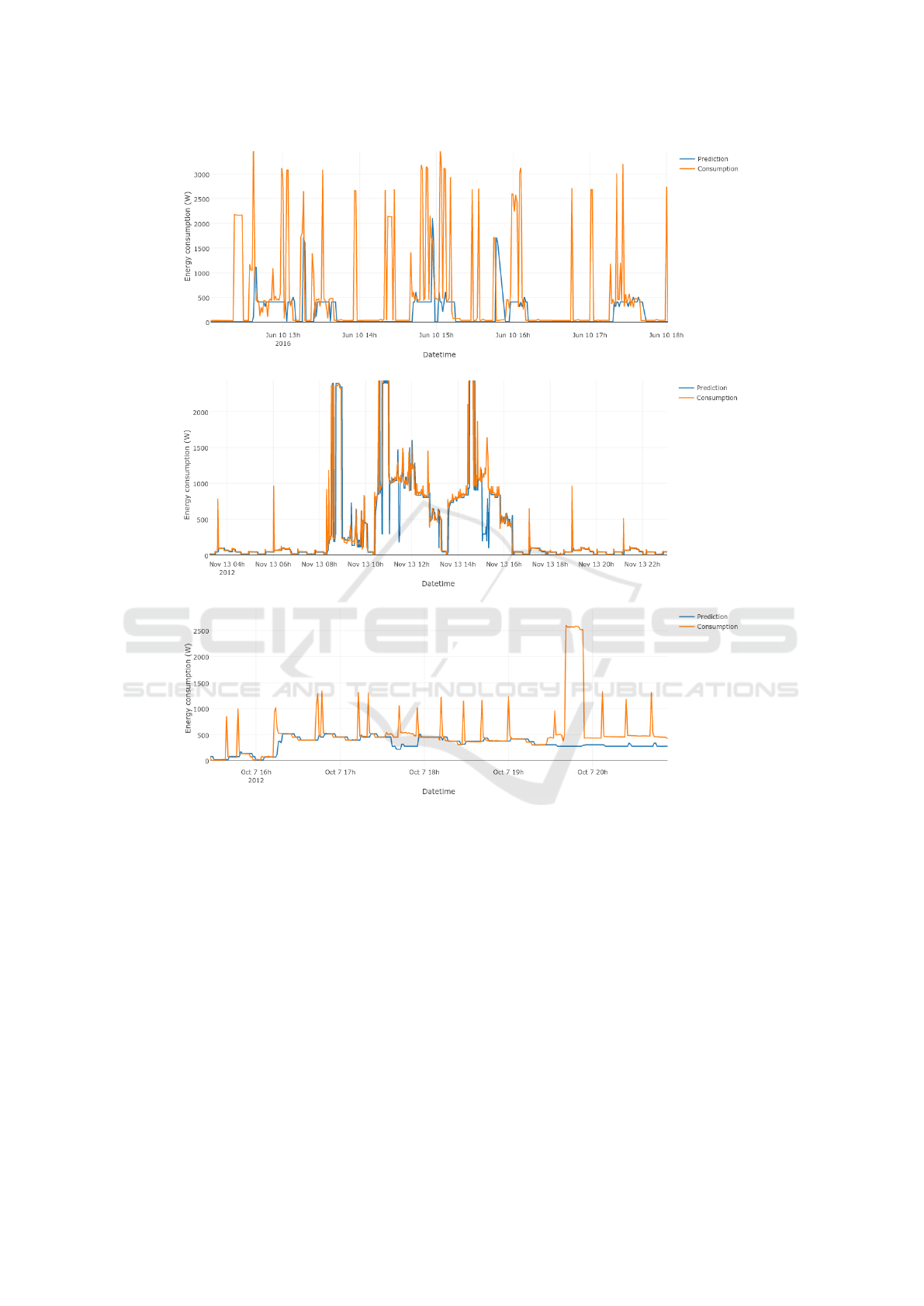
(a) RUG data set.
(b) ECO1 data set.
(c) ECO2 data set.
Figure 2: Energy consumption prediction for all data sets.
cision table, and a Bayesian Network to predict the
device usage for 1 hour and 24 hour intervals. While
they report the overall accuracy over 90% for the RE-
MODECE dataset (De Almeida et al., 2006), there is
no algorithm that generalizes well for all appliances;
the state prediction of lighting devices and oven appli-
ances perform better with the decision table approach,
while the state prediction for a washing machine is
most accurate when using the decision tree approach.
In (Zhang et al., 2016), Zhang et. al. proposed
a method using a weighted Support Vector Machine
with a differential evolution algorithm. Their goal is
to predict both the short-term and mid-term energy
consumption. The results of their experiments show a
MAPE of 5.843% for daily predictions and a MAPE
of 3.767% for half-hourly predictions. The authors
of (Jung et al., 2015) proposed an approach using
a Least Squared Support Vector Machine technique
for forecasting the daily energy usage of buildings.
To optimize the parameters of the model, DSOR-
CGA is applied, a hybrid of direct search optimiza-
tion and real-coded genetic algorithm. They report
an average Root Mean Square Error (RMSE) between
7.5994 and 11.1319, depending on the data set used.
In (Wang and Ding, 2015), the authors describe an an-
nual occupancy-based energy consumption prediction
method for offices, combining a Markov chain and the
Monte Carlo method. Their reported error rates vary
from 0.99% to 3.95%, depending on the office. The
authors of (Li et al., 2015) apply an Artificial Neural
Mining Sequential Patterns for Appliance Usage Prediction
31
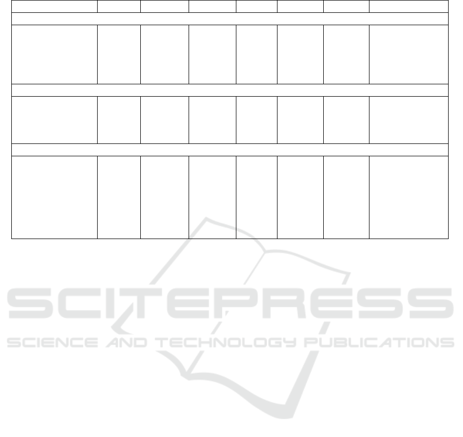
Table 6: Results for state prediction with failed sensor per device for all data sets.
Device Correct Corr. off Corr. on Wrong Dev. off Off cov. Same prediction
RUG data set
Screen 0.9996 0.9996 0 0.0005 0.9996 1 0.9998
Microwave 0.8861 0.08861 0 0.114 0.8861 1 0.8932
Boiler 0.9691 0.9691 0 0.031 0.9691 1 1
Coffee maker 0.8077 0.8077 0 0.1924 0.8077 1 1
Printer 0.7564 0.7564 0 0.2437 0.7564 1 0.8649
ECO1 data set
Fridge 0.598 0.607 0.4071 0.4021 0.6063 0.9563 0.636
Dryer 0.9606 0.9606 0 0.0395 0.9606 1 0.9623
Washing machine 0.9104 0.9104 0 0.0897 0.9104 1 0.9215
Freezer 0.4919 0.3835 0.623 0.5082 0.3806 0.5516 0.6754
ECO2 data set
Dishwasher 0.9842 0.9842 0 0.0159 0.9842 1 0.9901
Air exhaust 0.9886 0.9886 0 0.0115 0.9886 1 0.9979
Fridge 0.544 0.5619 0.5156 0.4561 0.532 0.6489 0.7482
Freezer 0.5518 0.4458 0.612 0.4483 0.409 0.3952 0.8107
Lamp 0.8247 0.8427 0 0.1754 0.8247 1 0.8344
TV 0.885 0.9959 0.7025 0.1151 0.732 0.8464 0.9998
Stereo 0.8932 0.8763 0.932 0.1069 0.6321 0.9675 0.9177
Network (ANN) to perform hourly predictions of a
building’s electricity consumption. They apply an im-
proved Particle Swarm Operation to adjust the ANN’s
structure, weights, and thresholds, ultimately result-
ing in a MAPE of 0.0162%. They also experiment
with a Genetic Algorithm-ANN and report a MAPE
of 0.00185%. These results improve the energy con-
sumption prediction using a normal ANN that deliv-
ers a MAPE of 0.0211%.
The work of Barbato et. al. (Barbato et al., 2011)
is closely related to our presented work. The authors
take a probabilistic approach to device state predic-
tions. Devices that were considered in their research
include: an oven, TV, boiler, and computer. For these
devices, they obtain a state prediction accuracy of
76%, 82%, 94%, and 88%, respectively. To compare
our approach to Barbato’s approach, we implement
their approach and evaluate it on an ECO data set.
We choose the ECO2 dataset, as it has the highest re-
liability: only 3% of the values are missing for the
fridge, freezer, dishwasher, TV, and stereo (Cicchetti,
2014). The evaluation of the approach on the ECO2
data set is shown in Table 7. When compared to our
approach (Table 4), we can see that in some cases the
performance is similar, while in general our approach
performs better. Barbato’s approach fails to identify
when the dishwasher and air exhaust are turned on.
For the fridge and freezer the results are closer to-
gether, though our approach performs approximately
10% to 15% better. The accuracy of the predictions
for the lamp come closest to ours, but once more their
approach struggles with the accuracy of ‘on’ predic-
tions. We observe a similar trend for the TV and
stereo.
In Tang et. al. (Tang et al., 2014), the authors also
consider the device states and estimate energy usage.
Based on the predicted device states, the authors esti-
mate power consumption using the rated power given
by hardware vendors. Their main concern is to break
the aggregated energy consumption to individual ap-
pliance for every timestamp, without learning the se-
quence of the device activation. Our work differs in
the way how energy consumption is predicted, as we
focus on individual devices instead of the aggregated
consumption.
5 CONCLUDING REMARKS
We proposed an approach based on a modified ver-
sion of Support-Pruned Markov Models to mine pat-
terns of device usage. We designed experiments in-
volving three data sets that represent real-world envi-
ronments. We achieved 87% accuracy in device usage
predictions over three different data sets. Moreover,
the approach is very reliable for devices that exhibit
a strong sequential pattern over time, achieving up to
99% accuracy in state predictions. For these selected
devices, the expected energy footprint is predicted
correctly with only a few Watts of error, resulting in
an accuracy of around 90%. We also demonstrated
that our approach can handle, to some degree, the us-
SMARTGREENS 2018 - 7th International Conference on Smart Cities and Green ICT Systems
32
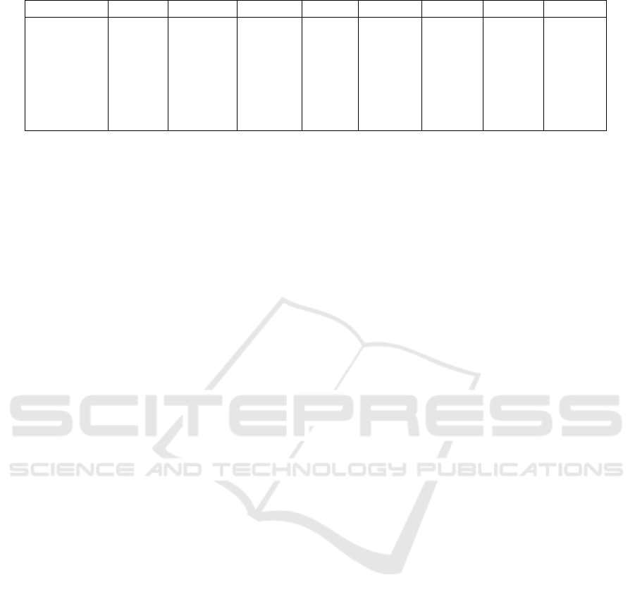
Table 7: State predictions results for Barbato et.al. approach (Barbato et al., 2011) on ECO2.
Device Correct Corr. Off Corr. on Wrong Dev. off Dev. on On cov. Off cov.
Dishwasher 0.9854 0.9854 0 0.0147 0.9854 0.0147 0 1
Air exhaust 0.962 0.9923 0.0155 0.0381 0.992 0.0081 0.0598 0.9693
Fridge 0.5004 0.6292 0.378 0.4997 0.6256 0.3745 0.5175 0.4902
Freezer 0.5146 0.4954 0.5281 0.4855 0.4817 0.5184 0.597 0.4259
Lamp 0.8987 0.9213 0.4768 0.1014 0.901 0.0991 0.2446 0.9706
TV 0.7156 0.835 0.4159 0.2845 0.7635 0.2366 0.501 0.7821
Stereo 0.6213 0.751 0.448 0.3788 0.6659 0.3342 0.5737 0.6452
age predictions of devices for which the sensor havew
failed. This is accurate for devices that have strong
sequential relationships amongst each other, that is,
these devices are often used together, or one after the
other. Cyclic and peak patterns, on the other hand, are
harder to predict with the proposed approach. This is
especially true when there is not a large quantity of
data available, therefore cyclic and peak patterns will
require a different set of techniques.
ACKNOWLEDGEMENT
Mathieu Kalksma thanks the Distributed Systems
Group at the University of Groningen for the opportu-
nity of and support while performing the presented re-
search. The work is partially supported by the Dutch
National Research Council Beijing Groningen Smart
Energy Cities Project, contract no. 467-14-037.
REFERENCES
Agrawal, R., Imielinski, T., and Swami, A. (1993). Min-
ing associations between sets of items in massive
databases. In Proceedings of the ACM-SIGMOD Int’l
Conference on Management of Data, pages 207–216.
Barbato, A., Capone, A., Rodolfi, M., and Tagliaferri, D.
(2011). Forecasting the usage of household appliances
through power meter sensors for demand management
in the smart grid. In 2011 IEEE International Con-
ference on Smart Grid Communications (SmartGrid-
Comm), pages 404–409.
Basu, K., Hawarah, L., Arghira, N., Joumaa, H., and Ploix,
S. (2013). A prediction system for home appliance
usage. Energy and Buildings, 67:668–679.
Beckel, C., Kleiminger, W., Cicchetti, R., Staake, T., and
Santini, S. (2014). The eco data set and the perfor-
mance of non-intrusive load monitoring algorithms. In
Proceedings of the 1st ACM International Conference
on Embedded Systems for Energy-Efficient Buildings
(BuildSys 2014). Memphis, TN, USA, pages 80–89.
ACM.
Cicchetti, R. (2014). Nilm-eval: Disaggregation of real-
world electricity consumption data. Master’s thesis,
Swiss Federal Institute of Technology Zurich.
De Almeida, A., Fonseca, P., Schlomann, B., Feilberg, N.,
and Ferreira, C. (2006). Residential monitoring to
decrease energy use and carbon emissions in europe.
In International Energy Efficiency in Domestic Appli-
ances & Lighting Conference.
Deshpande, M. and Karypis, G. (2004). Selective markov
models for predicting web page accesses. ACM Trans.
Internet Technol., 4(2):163–184.
EIA (2016). How is electricity used in u.s. homes?
https://www.eia.gov/tools/faqs/faq.php?id=96&t=3.
Accessed: 29-12-2017.
Georgievski, I., Degeler, V., Pagani, G. A., Nguyen, T. A.,
Lazovik, A., and Aiello, M. (2012). Optimizing en-
ergy costs for offices connected to the smart grid.
IEEE Trans. Smart Grid, 3(4):2273–2285.
Jung, H. C., Kim, J. S., and Heo, H. (2015). Prediction
of building energy consumption using an improved
real coded genetic algorithm based least squares sup-
port vector machine approach. Energy and Buildings,
90:76–84.
Kalksma, M. (2016). Mining household appliances patterns
by monitoring electric plug loads. Master’s thesis,
University of Groningen.
Li, K., Hu, C., Liu, G., and Xue, W. (2015). Building’s elec-
tricity consumption prediction using optimized artifi-
cial neural networks and principal component analy-
sis. Energy and Buildings, 108:106–113.
Pitkow, J. and Pirolli, P. (1999). Mining longest repeating
subsequences to predict world wide web surfing. Pro-
ceedings of USITS ’99: The 2nd USENIX Symposium
on Internet Technologies \& Systems, pages 139–150.
Pratama, A. R., Widyawan, Lazovik, A., and Aiello, M. (In
Press). Power-based device recognition for occupancy
detection. In Service-Oriented Computing - ICSOC
2017 Workshop.
Tang, G., Wu, K., Lei, J., and Tang, J. (2014). Plug and
play! A simple, universal model for energy disaggre-
gation. CoRR, abs/1404.1884.
Wang, Z. and Ding, Y. (2015). An occupant-based energy
consumption prediction model for office equipment.
Energy and Buildings, 109:12–22.
Zhang, F., Deb, C., Lee, S. E., Yang, J., and Shah, K. W.
(2016). Time series forecasting for building en-
ergy consumption using weighted Support Vector Re-
gression with differential evolution optimization tech-
nique. Energy and Buildings, 126:94–103.
Mining Sequential Patterns for Appliance Usage Prediction
33
