Development of a Remote Laboratory for Control-engineering

Education based on an Industrial Fluid Transport Platform

Danilo Pequeno, José Sérgio da Rocha Neto, Jaidilson Jó da Silva and Angelo Perkusich

Department of Electrical Engineering, Federal University of Campina Grande,

Aprigio Veloso Street, Campina Grande, Paraíba, Brazil

Keywords: Control Systems, Remote Laboratory, Computer Supported Education.

Abstract: This paper presents the development of a remote laboratory based on an industrial fluid transport platform.

The goal is to improve the control-engineering education using new technologies, saving equipment and

personnel for the institution and time and money for the remote students. The pilot plant was initially

developed for the study of fouling detection and adapted in this work for the development of a laboratory, in

which students and researchers can, over the Internet, perform experiments without any limitation of time and

location. The LabVIEW software was used to implement the Human-Machine Interface (HMI) through a

didactic interaction and the developed remote laboratory has been tested to be used in different disciplines.

1 INTRODUCTION

A very common problem that occurs in industrial

fluidic transport systems is the gradual accumulation

of organic or inorganic substances along the inner

surface of the tube in a process called fouling. It

happens slowly and it is typical of the chemical,

petroleum, food and pharmaceutical industries. This

is a serious problem because the fouling reduces the

internal diameter of the tube, as shown in Figure 1,

increasing the internal pressure, even the rupture of

the pipe (Rose, 1995).

Figure 1: The comparison between tubes with (left) and

without (right) fouling.

According to Mansoori (2002), pressure and flow

variables are directly associated with this process.

Consequently, these are the variables of interest for

monitoring and control system, in order to avoid the

fouling formation.

To promote the study of control systems and

industrial automation, a remote laboratory was

developed for an industrial fluid transport platform

available at the Electronic Instrumentation and

Control Laboratory (LIEC) in the Federal University

of Campina Grande (UFCG), Brazil.

This paper is organized as follows. In section 2, a

quick bibliographic review is made on industrial

control systems. Section 3 presents the experimental

platform under study with its all sensors and

actuators. In section 4, the results obtained for an on-

line experiment to test the laboratory are discussed.

Finally, section 5 summarizes a conclusion about the

remote laboratory developed and its applications for

undergraduate students on Electrical Engineering and

researchers on control systems.

2 CONTROL SYSTEMS

Control systems aim at a set of variables of a given

process behaving in a specific way in the domain of

time or frequency (Skogestad and Postlehwaite,

2005). Thus, the control system acts on manipulated

variables with the interest of controlling the output

variables of the process.

In general, a closed control loop is shown in

Figure 2. The controller acts on the process to be

Pequeno, D., Rocha Neto, J., Silva, J. and Perkusich, A.

Development of a Remote Laboratory for Control-engineering Education based on an Industrial Fluid Transport Platform.

DOI: 10.5220/0006666604730480

In Proceedings of the 10th International Conference on Computer Supported Education (CSEDU 2018), pages 473-480

ISBN: 978-989-758-291-2

473

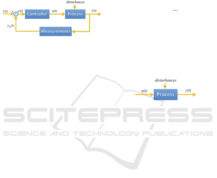
controlled by a manipulated variable u(t), calculated

form the error e(t) between the desired set point r(t)

and the measured value y

(t) of the output process

variable (Ogata, 2009). The process may be subject to

disturbances, which should be considered in the

design of the control system.

Figure 2: Control diagram in closed loop.

First of all, to design a control system, it is

necessary to identify the models of plant under study

through the modeling stage. Subsequently, the

controller is tuned according to the models and the

type of system.

2.1 Modeling

The identification of a mathematical model of the

system, which allows the design of controllers for the

plant, can usually be performed by two methods. In

the first, it is necessary to know the equations that

govern the physical phenomena associated to the

system. However, the theoretical method can result in

rather complex mathematical problems, so it is

common in industry to use the experimental method

(Ljung and Glad, 2016).

In the experimental method, the behavior of the

variables of interest is observed through the

application of known inputs that lead the outputs to

have a behavior already determined mathematically.

In practice, consecutive tests are performed on the

system and the input and output data are stored and

then processed in a specific software to adjust the

experimental curves obtained to the known

theoretical models.

2.2 PID Controller

The Proportional-Integral-Derivative (PID) action is

the most used in the industry and has been used

worldwide for industrial control systems. The

popularity of PID controllers can be attributed in part

to their robust performance over a wide range of

operating conditions and in part to their functional

simplicity, which allows engineers to operate them

directly (National Instruments, 2011).

As the name suggests, the PID controller is

composed of three parameters: Kp [dimensionless],

[seconds] is the integral time constant and T

[seconds] is the derivative time constant. Thus, the

PID controller can be represented according to the

Laplace Transform, as can be observed in the

Equation (1).













1 













 (1)

The parameters used to tune the PID controller

can be calculated by several techniques. The most

famous is the technique developed by Ziegler and

Nichols (1942).

2.3 SISO Systems

Systems that have a single input and a single output

variables are called SISO (Single Input Single

Output) systems, as can be seen in Figure 3.

Figure 3: SISO system diagram.

As can be observed, in these systems the output

variable y(t) can be directly controlled from the

manipulated variable u(t). Therefore, there will be

only one control loop. The mathematical model that

represents a process is called transfer function, and it

is a mathematical function that transforms the input

signal u(t) in the output y(t).

2.4 MIMO Systems

It is quite common to find, in real industrial processes,

control systems with more than one input and output.

These systems are called MIMO (Multiple Input

Multiple Output).

Figure 4 shows a MIMO system, in the frequency

domain, with two inputs and two outputs, also known

as the TITO (Two Inputs Two Outputs) system. It is

observed that both manipulated variables interact

directly with both outputs and therefore, there are

now four control loops, defined by four transfer

functions Hij(s), each one representing the influence

of input j on output i.

CSEDU 2018 - 10th International Conference on Computer Supported Education

474

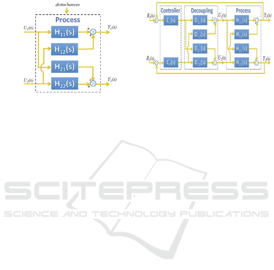
Figure 4: 2x2 MIMO system diagram.

MIMO control problems tend to be more complex

than SISO, as there are interactions in the process

between the output and manipulated variables.

Generally, a change in a manipulated variable (U

) will affect all the others output variables (Y

and

). Due to process interactions, the selection of the

best loop parity can be difficult.

In order to identify the best parity of the loops for

control (Y

and Y

or Y

and Y

several criteria were proposed like the Relative Gain

Array (RGA), proposed by Bristol (1966), and the

Relative Normalized Gain Array (RNGA) proposed

by He et al. (2009). These methods propose an

analysis of the force of interaction between the loops.

Once the control loops have been identified, it is

possible to proceed with the design of the PID

controllers, using a decentralized control structure.

Thus, each controller is designed as if the MIMO

system were a set of SISO systems.

2.4.1 Decoupling

When the interaction between the loops is not

significant, a decentralized controller, as presented

earlier, may be sufficient to ensure control of the

system. However, if the interactions are more

significant, a centralized controller using decoupling

is more appropriate, as suggested by Garrido et al.

(2011).

The decoupling is a matrix D of transfer functions,

inserted between the control matrix and the processes

matrix, as it can be observed in Figure 5. Its objective

is to compensate the interaction between the process

loops, so that the controller sees the Decoupling-

Process set as independent SISO systems.

Figure 5: TITO system with decoupling diagram.

3 EXPERIMENTAL PLATFORM

The experimental platform, shown in Figure 6, is

formed by galvanized steel tubes, being a 2” main

tube and another two 1” and 1 1/2” tubes used to

simulate disturbances on the system. The fluid used is

water, which is stored in a 100 liter tank.

3.1 PLC

A Programmable Logic Controller (PLC) can be

defined as an industrial computer that contains

hardware and software used to perform the control

functions. The PLC used in the platform is Siemens

S7-200, and includes a module with CPU 226, a

microcomputer, programming software STEP 7-

Micro/WIN SP9 version 4.0, whose programming is

done in Ladder language, and a PC/PPI

communication cable. In addition, there are a set of

EM231, EM232 and EM235 modules for reading and

triggering the analog inputs and outputs and the ASI

CP243-2 communication module.

3.2 Sensors

Each tube of the platform has its respective pressure

and flow sensors. The flow sensors are turbine

flowmeters and utilize the mechanical energy of the

fluid to rotate a rotor according to the flow. Then the

flow is measured from the rotational speed of this

rotor by means of an externally installed Hall Effect

sensor, Figure 7(a). This Signet Model 8550-1 sensor

also features a measurement transmitter and display

panel, Figure 7(b), powered by a 24V DC source, and

it provides flow ratings from 3 to 38 LPM (liters per

minute).

Development of a Remote Laboratory for Control-engineering Education based on an Industrial Fluid Transport Platform

475

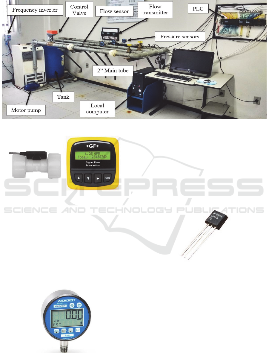
Figure 6: Photograph of the experimental platform.

(a) (b)

Figure 7: (a) Flow sensor; (b) Flow transmitter.

The pressure sensors, as shown in Figure 8, are of

the strain gauge type and are based on the principle of

varying the resistance of a wire. Through the

interconnection of four strips in a Wheatstone bridge

circuit, adjusted and balanced to the initial condition,

it is possible to measure the pressure by means of the

unbalance proportional to the variation of the

resistance of each strip. This instrument, model 2274-

XAO from Ashcroft, offers digital display in 9 units:

psi, mmHg, Pol, Hg, ft, Mpa, KPa, kgf/cm

and mBar.

Figure 8: Pressure sensor with an integrated transmitter.

There is also a temperature sensor LM35, Figure

9, of TO-92 encapsulation submerged within the tank.

This is a precision sensor, manufactured by National

Semiconductor, which has a linear voltage output

relative to the temperature when powered by a single

(4-20V DC) or symmetrical voltage source. This

sensor does not require any external calibration to

provide its measurements, having temperature values

ranging from ¼°C or even ¾°C, operating within a

temperature range of -55°C to 150°C.

Figure 9: Temperature sensor.

3.3 Actuators

Regarding the actuators, the main tube has a control

valve, model G250 from manufacturer Belimo. It is a

two-way globe valve with a single seat and a nominal

diameter of 2”. This is a valve with linear motion, as

it has a plug attached to a rod that moves linearly to

the seat, varying the area of passage of the fluid.

The control of the valve is done by an electric

actuator, model NVF24-MTF-E-US of the same

manufacturer. This actuator converts the electrical

power provided by the controller into mechanical

power, changing the relative position between the

plug and the seat. In a fault condition, the valve is

CSEDU 2018 - 10th International Conference on Computer Supported Education

476

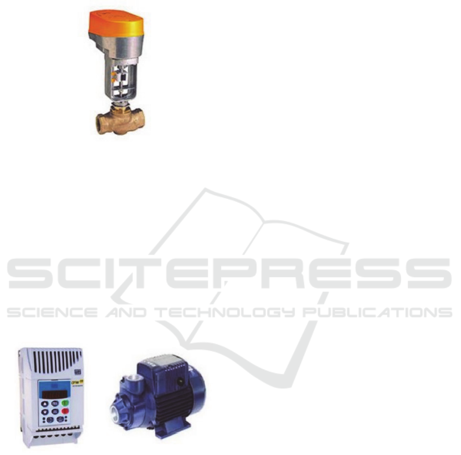
fully closed in order to guarantee the safety of the

process. It is powered by a 24V DC power supply

with 5.5W power. The valve and the actuator are

shown in Figure 10.

Figure 10: Control valve and its electrical actuator.

As for the other actuator present on the platform,

there is a frequency inverter, model CFW 080026

S2024 PSZ from the manufacturer WEG, Figure

11(a), which acts on the speed control of a motor

pump, based on frequency variation. The inverter has

a single-phase power supply 200-240V AC, 0.5CV

power, 4 poles with 220V three-phase output. It also

has four digital inputs and one analog input for

communication with the PLC and a resolution of

0.01Hz for frequencies up to 100Hz.

The motor pump, Figure 11(b), is a centrifugal

pump, model P500T hydro bloc from manufacturer

KSB. It has power of 0.5CV in 3500RPM, 2 poles and

three-phase power supply 220 V.

(a) (b)

Figure 11: (a) Frequency inverter; (b) Motor pump.

4 RESULTS

The experience in Engineering teaching has shown

that a complementary approach combining

theoretical and practical activities is vital for effective

and efficient learning (Callaghan et al., 2005). In this

sense, engineering education has incorporated

advances in technologies to promote expected

outcomes and a successful understanding.

4.1 HMI

In this section, the HMI is presented, which allows

on-line interaction between students and the platform,

as well as the results of an experiment performed

through remote access.

In order to implement the remote access to the

study platform, a HMI was developed, allowing a

didactic interaction between the students and the

platform. The tool used was LabVIEW (Laboratory

Virtual Engineering Workbench) software, which is a

development environment for a graphical

programming language developed by National

Instruments.

Programs in LabVIEW are called Virtual

Instruments (VI). Each VI has three components: a

block diagram, a front panel and a connection panel.

The software also has the Remote Panels tool that

converts the application into a remote laboratory,

where the HMI created for the purpose of controlling

and monitoring industrial plant is fully accessible by

the remote user.

The developed interface is divided in three tabs

and in all of them the user can download the collected

data. The first is the Instrumentation tab, Figure 12(a),

in which the user has direct access to all sensors and

actuators present on the platform. From this tab, the

user can perform tests to the industrial process

modeling, to deal with data in a specific software, to

identify the mathematical models and then design the

PID controllers and the decoupling.

The SISO tab, Figure 12(b), allows the user to

perform the SISO control of the experimental

platform loops, while the Multivariable Control tab,

Figure 12(c), allows the user to perform the MIMO

control of the system. Thus, in both tabs the user

enters the parameters of the controllers and

decoupling, defines a set point for the variables of

interest and monitors, in real time, the behavior of the

control system implemented.

Development of a Remote Laboratory for Control-engineering Education based on an Industrial Fluid Transport Platform

477

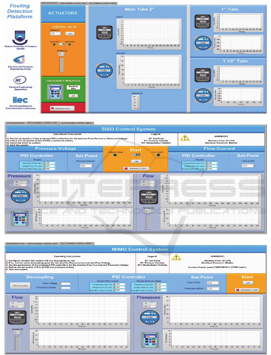
(a)

(b)

(c)

Figure 12: (a) Instrumentation tab; (b) SISO tab; (c) MIMO tab.

CSEDU 2018 - 10th International Conference on Computer Supported Education

478

4.2 Experimental Results

Step response tests were performed in the four loops

of the system: Flow-Voltage, Flow-Current,

Pressure-Voltage and Pressure-Current. The

manipulated variables voltage and current correspond

to the voltage applied to the frequency inverter and

the current applied to the actuator of the control valve,

respectively. The collected data were processed in the

Matlab software and the four identified FOPDT (First

Order Plus Dead Time) models are presented in Table

Table 1: Identified Models.

Loop Transfer Function Model

Flow-Voltage













0.86

9.97  1



.

Flow-Current











1.18

18.79  1



6.08

Pressure-Voltage













0.05

5.20  1



.

Pressure-Current













0.04

10.82  1



.

From the models presented, the analysis of the

interaction between the loops of the system was

performed according to the RGA and RNGA criteria,

presented previously. Both methods indicate that the

best parity for control is obtained using the Current-

Flow and Pressure-Voltage loops.

Once the mathematical models of the system were

know and the loops for control were defined, the PID

controllers were designed. The tuning method used

was the one proposed by Ziegler and Nichols,

previously mentioned. The parameters obtained for

the controllers are presented in Table 2.

Table 2: PID Controllers.

Loop Kp T

Flow-Current 3.71 12.17 3.04

Pressure-Voltage 0.62 20.02 5.01

A set of static decoupling, presented in Table 3,

were also calculated for the MIMO control system,

according to Garrido et al. (2011).

Table 3: Static Decoupling.

Decoupling Static Value

1.0000

-0.7276

-0.9020

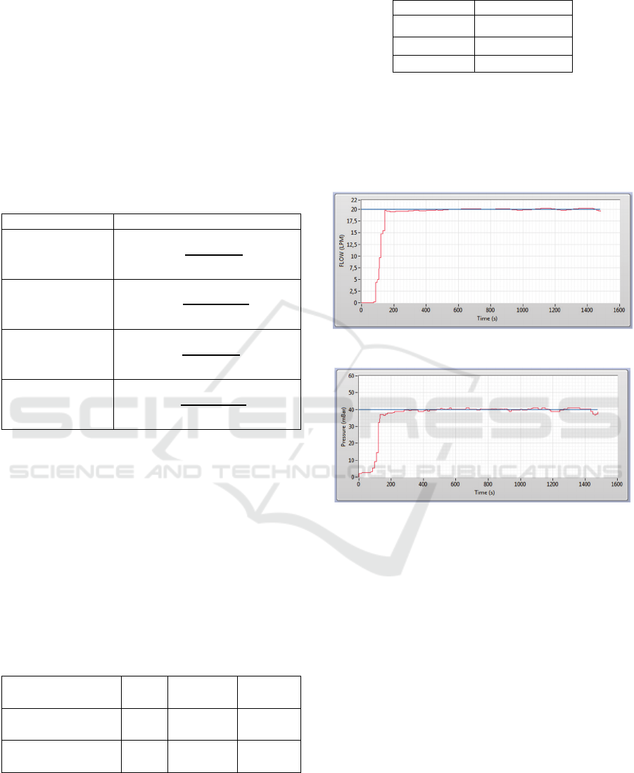
Using the remote access to the platform,

experiments were performed to study the MIMO

control system using static decoupling. In Figures 13

and 14, it is possible to observe the behavior, in real

time, of the system implemented for the Flow-Current

and Pressure-Voltage loops, respectively.

Figure 13: Flow-Current control response.

Figure 14: Pressure-Voltage control response.

This whole experiment was executed via remote

access. It can be noticed that from the initial data

collected it was possible to analyze the process and

design a control system. When implemented, the

control system ensured that the platform operated

within flow and pressure values defined by the user.

4.3 Remote Laboratory

According to National Instruments (2002), a remote

laboratory can be defined as a computer controlled

laboratory, which can be accessed and controlled

externally trough different communication methods.

Thus, a remote lab can be an experiment or process

executed locally on the LabVIEW platform, but with

the ability to be monitored and controlled over the

Internet using the developed HMI.

During the remote access, data acquisition

continues on the local computer, but the remote user

Development of a Remote Laboratory for Control-engineering Education based on an Industrial Fluid Transport Platform

479

has full control over the platform. Other users may try

to access the interface monitor of the application in

progress, but only one client can control the

application at a time. At any time during this process,

the local machine operator can take control over the

application.

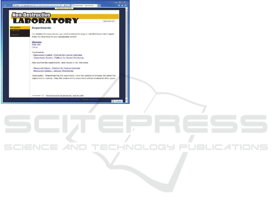
The web page of the developed remote laboratory

is shown in Figure 15, is better explained in Melo et

al. (2012).

Figure 15: Non-Destructive Laboratory web page.

5 CONCLUSIONS

In this paper it was presented the implementation of a

remote laboratory for the study of control systems and

industrial automation. One of the great advantages of

the experimental platform used is that different

control strategies can be implemented for both SISO

and MIMO systems in a single environment.

The incorporation of new technologies applied to

teaching, especially to distance education, gives to

students the opportunity to interact at any time with a

real laboratory. Thus, the laboratory not only

illustrates the concepts acquired in theory, but it also

allows students to see how unexpected events and

natural phenomena affect real-world measurements

and control algorithms.

The developed laboratory was tested, as presented

in the subsection 4.2, with an experiment on the

control of the multivariable system with PID

controllers and decoupling devices. However, the

present experiment is only one of many others that

can be performed by students of the disciplines of

Analog Control, Electronic Instrumentation and

Industrial Automation Systems modules in order to

complement the theory seen in the classroom.

ACKNOWLEDGEMENTS

The authors would like to thank the National Council

for Scientific and Technological Development

(CNPq) for financial support and everyone from the

Control and Eletronic Instrumentation Laboratory

(LIEC –UFCG) who supported the development of

this work.

REFERENCES

Bristol, E. (1966). On a New Measure of Interaction for

Multivariable Process Control. IEEE Transactions on

Automatic Control. IEEE, pp. 133-134.

Callaghan, M., Harkin, J., Gueddari, M., McGinnity, T. and

Maguire, L. (2005). Client-Server Architecture for

Collaborative Remote Experimentation. Proceedings of

the Third International Conference on Information

Technology and Applications. Sydney: IEEE.

Garrido, J., Vázquez, F. and Morilla, F. (2011). Generalized

Inverted Decoupling for TITO processes. 18th IFAC

World Congress. Milano, pp. 7535-7540.

He, M., Cai, W., Ni, W. and Xie, L. (2009). RNGA based

control system configuration for multivariable

processes. Journal of Process Control, 19. ELSEVIER,

pp. 1036-1042.

Ljung, L. and Glad, T. (2016). Modeling and Identification

of Dynamic Systems. Lund: Studentitteratur, pp. 19-27.

Mansoori, G. Ali. (2002). Physicochemical Basis of

Fouling Prediction and Prevention in the Process

Industry. Journal of the Chinese Institute of Chemical

Engineers. Vol. 33, No. 1, pp. 25-31.

National Instruments. (2002). Distance-Learning Remote

Laboratories using LabVIEW. Available at:

http://discoverlab.com/References/WP238.pdf

[Acessed 10 Sept. 2017].

National Instruments. (2011). PID Theory Explained.

Available at: http://www.ni.com/white-paper/3782/en

[Acessed 09 Sept. 2017].

Ogata, K. (2009). Modern Control Engineering. 5th ed.

Upper Saddle River: Prentice Hall.

Melo, T. R., Bezerra, M. M., Silva, J. J. and Neto, J. S. R.

(2012). Experimental Tests in non-destructive

laboratory – On-line Experiment: Monitoring Sensors.

In Proceedings of the 4th International Conference on

Computer Supported Education – Volume 2: CSEDU,

pp. 345-348.

Rose, J. (1995). Recent advances in guided wave NDE. In:

Proceedings of the IEEE Ultranic Symposim. Seattle:

IEEE, pp. 761-770.

Skogestad, S. and Postlehwaite, I. (2005). Multivariable

Feedback Control: Analysis and Design. Hoboken:

Wiley, pp. 2-5.

Ziegler, J. and Nichols, N. (1942). Optimum Settings for

Automatic Controllers. Journal of Dynamic Systems,

Measurement, and Control, 115(2B), pp. 220-222.

CSEDU 2018 - 10th International Conference on Computer Supported Education

480