Environmental Metagenome Classification for Soil-based
Forensic Analysis
Jolanta Kawulok and Michal Kawulok
Institute of Informatics, Silesian University of Technology, Akademicka 16, 44-100, Gliwice, Poland
Keywords:
Metagenomes, Environmental Classification, CoMeta, Forensic Analysis, Soil Sample.
Abstract:
Metagenome analysis makes it possible to extract essential information on the organisms that have left their
traces in a given environmental sample. In some cases, it is sufficient to determine the origin of an environmen-
tal sample, rather than being able to accurately identify the organisms living there (which may be a challenging
task). For example, in forensic soil analysis, it could be possible to confirm or exclude that a defendant was
present in a certain place by comparing a soil sample acquired from his belongings against the samples derived
from a variety of places (including the suspected place). In this paper, we present a method to identify the
environmental origins of metagenomic reads by comparing them with entire metagenomic collections derived
from reference samples. For this purpose, we exploit our CoMeta program, which allows for fast classification
of metagenome samples, and we apply it to classify the extracted soil metagenomes to various collections of
soil samples. The experimental results reported in this paper indicate that the proposed approach is effective,
which allows us to outline the future research pathways to extend and improve our method.
1 INTRODUCTION
Nowadays, we may witness rapid development of the
methods for analysis of metagenomic reads, which
are sets of DNA fragments, represented as strings of
nucleotide symbols, derived from microbes living in a
given environment. The analysis of samples acquired
from explored places is aimed at answering the fol-
lowing questions: “Who is out there?”, “How much
of each?”, “What are their proportions?”, “What are
they doing?”, and “In what conditions appear?” (Han-
delsman, 2004; Simon and Daniel, 2011). Answer-
ing these questions requires solving two classification
tasks, which respond to particular bioinformatic prob-
lems, falling into two major categories, namely super-
vised and unsupervised classification.
1.1 Related Work
Supervised classification of metagenomic reads con-
sists in comparing presented DNA fragments (termed
as a query sample) against a set of reference se-
quences, and the query sample is assigned to one
of these sequences (or to none of them). There are
many programs for sequence classification, which can
be divided into (i) composition-based and (ii) sim-
ilarity search ones. The composition-based meth-
ods compare the features extracted from the refer-
ence sequences, such as the frequency, with which
certain substrings of a given length k occur in an an-
alyzed sequence (Weitschek et al., 2014). A num-
ber of methods are employed to classify the ex-
tracted feature vectors, including interpolated Markov
models, support vector machines (Patil et al., 2011),
k-nearest neighbors (Weitschek et al., 2015), ran-
dom forests (Chen and Lonardi, 2009), or naive
Bayes classifier (Rosen et al., 2011). In the sim-
ilarity search methods, the reads are compared di-
rectly with the reference sequences—they include
MEGAN (Huson et al., 2007) and CARMA3 (Ger-
lach and Stoye, 2011) programs. There are also some
approaches to combine the elements of both strate-
gies (e.g., CoMeta (Kawulok and Deorowicz, 2015),
LMAT (Ames et al., 2013) or Kraken (Wood and
Salzberg, 2014)).
Comparing thousands of DNA fragments against
a huge database is very time consuming. Therefore,
in order to effectively search the databases, the simi-
larity measure between the DNA fragments is defined
and computed employing specific optimization tech-
niques, including compression and indexing. Based
on the similarity between the reads and the refer-
ence sequences, the reads may be classified into some
groups of the reference sequences, defined according
182
Kawulok, J. and Kawulok, M.
Environmental Metagenome Classification for Soil-based Forensic Analysis.
DOI: 10.5220/0006659301820187
In Proceedings of the 11th International Joint Conference on Biomedical Engineering Systems and Technologies (BIOSTEC 2018) - Volume 3: BIOINFORMATICS, pages 182-187
ISBN: 978-989-758-280-6
Copyright © 2018 by SCITEPRESS – Science and Technology Publications, Lda. All rights reserved

to the objective of the study. Depending on the main
goal of the analysis, which determines the way the
reference groups are defined, supervised classification
of metagenomic data can be broken down as follows:
• Taxonomic classification—each reference group
contains DNA fragments of organisms assigned
to the same taxon, whose rank may span from the
superkingdom to the species (Gerlach and Stoye,
2011; Bazinet and Cummings, 2012).
• Functional classification—a reference group con-
tains the DNA fragments that enable the microor-
ganisms fulfill a certain function (e.g., degrada-
tion of petroleum alkanes) (Bazinet and Cum-
mings, 2012; Kennedy et al., 2011).
• Environmental classification—each reference
group is formed with a metagenomic sample (or
samples) acquired from a certain environment.
The goal of such classification scheme is to
determine the characteristics of the environment,
rather than identifying the organisms living there.
It is worth noting that the reference sequences
within each reference group do not have to
be annotated (assigned to specific species or
taxonomic units), which facilitates the procedure
in many cases.
The metagenomic reads may also be analysed
without using any reference sequences, which is re-
ferred to as unsupervised classification. In such sce-
nario, the obtained reads are grouped into opera-
tional taxonomic units (OTUs) based on their mu-
tual similarities. This process is termed as binning—
among many applications, it is used for analysing
the proportion between different groups of organisms.
Here, similar optimization techniques (like compres-
sion and indexing of the sequences) can also be used
so as to accelerate the comparison process.
1.2 Contribution
In this paper, we address a problem of environmental
classification, which has a wide variety of potential
practical applications. Here, we focus on analysing
soil samples for forensic purposes—the goal is to con-
firm or reject a hypothesis that a certain defendant
visited a specific place—soil traces acquired from his
belongings can be verified against a set of samples ac-
quired from a variety of places. Our contribution lies
in comparing the samples by measuring their simi-
larity directly in the space of the metagenome reads.
This is in contrast to earlier research in this field
(Khodakova et al., 2014), in which the samples were
first analysed to identify the microorganisms, whose
genomes are present in these samples, and then the
similarity was assessed by comparing the identified
species. Importantly, in our approach, we do not need
a reference database that is necessary to identify the
microorganisms. Although in this work we validate
our method for forensic data analysis, the developed
solution is generic and may be adopted to a differ-
ent scenario of environmental metagenomic classifi-
cation. Our main point here is that the knowledge
of particular species is not necessary to recognize the
origin of the sample.
1.3 Paper Structure
The paper is structured as follows. Section 2.1
presents the metagenomic sets we use for validation,
whilst Section 2.2 describes how they are exploited
in the classification process. Section 3 presents the
results of experimental validation, and Section 4 con-
cludes the paper.
2 MATERIALS AND METHODS
2.1 Metagenomic Sampling
For testing our method, we decided to select samples
derived from the soils. Owing to the large microbial
diversity of soil, soil sample classification can serve
as a powerful tool for forensic soil examination. Soil
can be found on items submitted for forensic analysis.
Soil sticks under fingernails, tools, weapons or cloths
and it can be transferred during the commission of a
criminal act (Khodakova et al., 2014).
We selected soil samples derived from four lo-
cations examined within three different projects.
The data sets were downloaded from EBI Metage-
nomics website
1
. Two of these projects were con-
ducted in the USA—in Alabama and Massachusetts
states (Stewart et al., 2011). Soil samples from the
third project were collected from two different sites
in Adelaide in South Australia (Khodakova et al.,
2014). These locations are approximately 3 km from
each other. The most relevant characteristics of these
metagenomic sets are presented in Table 1. The sets
contain 2 or 3 samples, each of which consists of hun-
dreds of thousands metagenomic reads.
2.2 Research Methodology
There are a number of tools for comparing metage-
nomic data, out of which for our study we selected our
1
Available at https://www.ebi.ac.uk/metagenomics (ac-
cessed on 9th October 2017)
Environmental Metagenome Classification for Soil-based Forensic Analysis
183

CoMeta (Classification of Metagenomes) program
2
(Kawulok and Deorowicz, 2015) due to its versatil-
ity and ease of use. Most of the existing tools are
intended for a specific application, and we found it
difficult (if feasible at all) to deploy some of them for
a different purpose. Basically, CoMeta has been de-
signed for fast and accurate classification of reads ob-
tained after sequencing entire environmental samples
and it allows a database to be built without any re-
strictions. The similarity (termed the match score) be-
tween the query read and each group (class) of the ref-
erence sequences is determined by counting the num-
ber of the nucleotides in those k-mers (i.e., all sub-
strings in the sequence of length k), which occur both
in the read and in the group. The read is classified to
that group, for which the match score is the largest.
We organize the reference sequences into the groups
of DNA sequences acquired from soils derived from
various places (each of these places is treated as a sep-
arate class). In this way, a new metagenomic sample
is classified to one of the created classes.
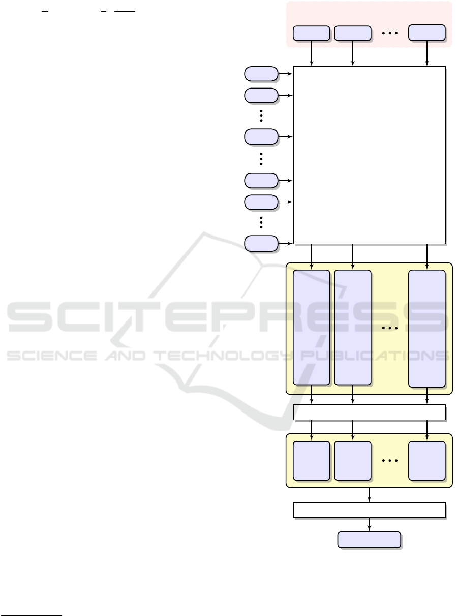
A simplified diagram of our classification scheme
is shown in Figure 1. We have built N = 10 separate
sets of k-mers from the reads of metagenomic data
acquired from each sample in the reference (train-
ing) set. The reads acquired from a given sample
were compared only to other samples. The reads
derived from a query sample are compared against
the number of groups equal to the number of all in-
vestigated samples in the reference set (in the pre-
sented experiment—N − 1 = 9). The set of reference
sequences consists of n
I
+ n
I
I + ··· + n
N
databases,
wherein n
I
ones are derived from first metagenomic
set (D
I1
, D
I2
, ..., D
In
I
), n
I
I from the second, and so on.
They are compared with q reads derived from a query
sample. The result of a single matching is termed
the match rate score (Ξ
Ri j
). During the intermediate
analysis, each read is attributed to one of the created
groups after exceeding a certain threshold defined for
each group; otherwise it is marked as unknown (U).
Finally, the initial assignment of each read and collec-
tively all match rate scores (yellow boxes in the dia-
gram) are completely analyzed and the query sample
is classified to the appropriate class.
3 RESULTS
At the beginning of our experimental validation, we
verified the correctness of our framework. For this
purpose, we built four metagenomic databases—one
2
Available at https://github.com/jkawulok/cometa (ac-
cessed on 9th October 2017)
D
I1
D
I2
D
In
I
D
N 1
D
N 2
D
N n
N
Comparison
R
1
R
2
R
q
Query Sample
Ξ
R1I1
Ξ
R1I2
.
.
.
Ξ
R1In
I
Ξ
R1N 1
Ξ
R1N 2
.
.
.
Ξ
R1N n
N
Ξ
R2I1
Ξ
R2I2
.
.
.
Ξ
R2In
I
Ξ
R2N 1
Ξ
R2N 2
.
.
.
Ξ
R2N n
N
Ξ
RqI1
Ξ
RqI2
.
.
.
Ξ
RqIn
I
Ξ
RqN 1
Ξ
RqN 2
.
.
.
Ξ
RqN n
N
Intermediate analysis
I/II/
. . .
/N/U
I/II/
. . .
/N/U
I/II/
. . .
/N/U
Intermediate analysis
Complete analysis
I/II/. . . /N/U
Figure 1: The processing pipeline for metagenomic reads
classification to the one of the created classes.
for each place. Subsequently, we compared each sam-
ple with all of them so as to make sure that every read
is properly assigned to the environment which it came
from. In the next step, the databases of each sample
BIOINFORMATICS 2018 - 9th International Conference on Bioinformatics Models, Methods and Algorithms
184

Table 1: Metagenomic data sets.
No. Project ID Site
Number Average number
of samples of reads
1 SRP016569 Bankhead National Forest (Alabama, US) 2 322 856
2 SRP005264
(Stewart et al.,
2011)
Harvard Forest (Massachusetts, US) 2 1 182 612
3A ERP004852
(Khodakova
et al., 2014)
1st Adelaide park (AU) 3 402 093
3B ERP004852
(Khodakova
et al., 2014)
2nd Adelaide park (AU) 3 330 957
were created separately. As a result, we received 10
databases. At first, we used them also by comparing
each read against all the databases. We have achieved
the same effect as in the previous case—100% of the
reads were assigned correctly. This was expected,
given that CoMeta uses an approximate matching of
two sequences, hence for each read we received the
exact matching to that very read that was found in the
sample of origin.
In order to validate the classification method, it
was necessary to compare the reads with the sets,
in which they were not located. This approach was
already described in Section 2.2—each read derived
from one of N = 10 samples was compared with
N − 1 = 9 databases.
Figure 2 shows how many percent of the reads
were matched to each location. If a read from the first
sample in a given location is correctly matched to its
location, then it means that the read has been assigned
to a database built on the second (and/or third) sam-
ple (samples) from that location (it is not compared
with other reads from its sample of origin). We mea-
sure the classification accuracy at a sample level—we
consider a sample as correctly assigned when the ma-
jority of the reads from that sample are attributed to
the correct location.
From Figure 2, it can be noticed that 7 out of 10
samples are classified correctly, which generally con-
firms that our approach is correct. It is worth not-
ing that only the samples from the 2nd Adelaide park
location were incorrectly classified—actually, all of
them were assigned to the 1st Adelaide park loca-
tion. Certainly, these samples are similar to each other
due to small distance between these locations, but it
is worth noting that the first location contains more
samples than the second one (see Table 1), so the
classification could be biased towards the first loca-
tion. We will address this problem by (i) introducing
the weights according to the cardinality of a sample
and (ii) rejecting (or reducing the impact) of the reads
classified to several samples. Basically, if a read is
assigned to only one sample, than it may be consid-
ered as a more specific indicator of a certain location
than another read that is matched to several locations.
In our initial study reported here, we do not take into
account the uniqueness of the reads and we suspect
that this could be the main reason for the misclassified
samples observed for the 2nd Adelaide park location.
Overall, these results clearly indicate that it is feasi-
ble to identify the origin of a sample without the need
for identifying the microorganisms that have left their
traces in that sample.
4 CONCLUSIONS AND FUTURE
WORK
In this paper, we proposed a method for classify-
ing metagenomic reads to the reference environmen-
tal groups. The presented experimental results proved
the feasibility of our approach and it may be consid-
ered for the purpose of forensic analysis. A very im-
portant advantage of our approach lies in measuring
the sample similarity at the reads level without the
necessity to understand the contents of these samples.
We also consider a hybrid method to exploit both the
information on the organisms identified in the sam-
ples, as well as to benefit from the reads-level similar-
ity. Hence, if some organisms are identified in a sam-
ple, then this can be utilized during classification, but
information of the unknown organisms whose traces
are found in a sample, will not be lost.
Our ongoing research is aimed at improving the
environmental classification engine, following our
observations reported earlier in Section 3. Instead of
counting the matching reads, we intend to analyse the
matches in terms of their uniqueness. Also, we plan
to improve the testing methodology and split the sam-
ples into smaller parts (so as to analyze the classifica-
Environmental Metagenome Classification for Soil-based Forensic Analysis
185

1st Adelaide park 2nd Adelaide park
(Soil metagenomes (Soil metagenomes Harvard Forest Bankhead National Forest
place-1) place-2)
1
st
sample
correctly classified as
1st Adelaide park
incorrectly classified as
1st Adelaide park
correctly classified as
Harvard Forest
correctly classified as
Bankhead National
Forest
2
nd
sample
correctly classified as
1st Adelaide park
incorrectly classified as
1st Adelaide park
correctly classified as
Harvard Forest
correctly classified as
Bankhead National
Forest
3
rd
sample
correctly classified as
1st Adelaide park
incorrectly classified as
1st Adelaide park
Figure 2: Results of environmental classification.
tion scores at a lower-than-sample level).
The second important direction of our future work
is concerned with applying the proposed framework
to solve other practical challenges in medicine, en-
gineering, agriculture, and ecology. In particular,
we plan to compare the performance of our method
against the state of the art (Turnbaugh et al., 2009;
Cui and Zhang, 2013) in diagnostics. Here, the
metagenome is exploited to confirm or exclude a spe-
cific disorder for a patient, whose metagenomic sam-
ple is compared against two groups of metagenomic
reads, derived from (i) positively diagnosed patients
and (ii) a control group.
ACKNOWLEDGEMENTS
This research was supported in part by PL-Grid In-
frastructure. This work was supported by the Pol-
ish National Science Centre under the project DEC-
2015/19/D/ST6/03252 .
BIOINFORMATICS 2018 - 9th International Conference on Bioinformatics Models, Methods and Algorithms
186

REFERENCES
Ames, S., Hysom, D. A., Gardner, S. N., Lloyd, G. S.,
Gokhale, M. B., and Allen, J. E. (2013). Scalable
metagenomic taxonomy classification using a refer-
ence genome database. Bioinformatics, 29(18):2253–
2260.
Bazinet, A. L. and Cummings, M. P. (2012). A comparative
evaluation of sequence classification programs. BMC
Bioinformatics, 13(1):1–13.
Chen, J. Y. and Lonardi, S. (2009). Biological data mining.
CRC Press.
Cui, H. and Zhang, X. (2013). Alignment-free supervised
classification of metagenomes by recursive SVM.
BMC Genomics, 14(1).
Gerlach, W. and Stoye, J. (2011). Taxonomic classification
of metagenomic shotgun sequences with CARMA3.
Nucleic Acids Research, 39(14):E91–E101.
Handelsman, J. (2004). Metagenomics: application of ge-
nomics to uncultured microorganisms. Microbiol Mol
Biol Rev., 68(4).
Huson, D. H., Auch, A. F., Qi, J., and Schuster, S. C. (2007).
MEGAN analysis of metagenomic data. Genome Re-
search, 17(3):377–386.
Kawulok, J. and Deorowicz, S. (2015). CoMeta: Clas-
sication of metagenomes using k-mers. PLoS ONE,
10(4):e0121453.
Kennedy, J., O’Leary, N., Kiran, G., Morrissey, J., O’Gara,
F., Selvin, J., and Dobson, A. (2011). Functional
metagenomic strategies for the discovery of novel en-
zymes and biosurfactants with biotechnological appli-
cations from marine ecosystems. Journal of Applied
Microbiology, 111(4):787–799.
Khodakova, A. S., Smith, R. J., Burgoyne, L., Abarno, D.,
and Linacre, A. (2014). Random whole metagenomic
sequencing for forensic discrimination of soils. PloS
one, 9(8):e104996.
Patil, K. R., Haider, P., Pope, P. B., Turnbaugh, P. J., Mor-
rison, M., Scheffer, T., and McHardy, A. C. (2011).
Taxonomic metagenome sequence assignment with
structured output models. Nature Methods, 8(3):191–
192.
Rosen, G. L., Reichenberger, E. R., and Rosenfeld, A. M.
(2011). NBC: The naive Bayes classification tool
webserver for taxonomic classification of metage-
nomic reads. Bioinformatics, 27(1):127–129.
Simon, C. and Daniel, R. (2011). Metagenomic Analy-
ses: Past and Future Trends. Appl Environ Microbiol,
77(4):1153–1161.
Stewart, F. J., Sharma, A. K., Bryant, J. A., Eppley,
J. M., and DeLong, E. F. (2011). Community tran-
scriptomics reveals universal patterns of protein se-
quence conservation in natural microbial communi-
ties. Genome biology, 12(3):R26.
Turnbaugh, P. J., Hamady, M., Yatsunenko, T., Cantarel,
B. L., Duncan, A., Ley, R. E., Sogin, M. L., Jones,
W. J., Roe, B. A., Affourtit, J. P., Egholm, M., Henris-
sat, B., Heath, A. C., Knight, R., and Gordon, J. I.
(2009). A core gut microbiome in obese and lean
twins. Nature, 457(7228):480–484.
Weitschek, E., Fiscon, G., Fustaino, V., Felici, G., and
Bertolazzi, P. (2015). Clustering and classification
techniques for gene expression profile pattern analy-
sis. Pattern Recognition in Computational Molecular
Biology: Techniques and Approaches, page 347.
Weitschek, E., Santoni, D., Fiscon, G., De Cola, M. C.,
Bertolazzi, P., and Felici, G. (2014). Next generation
sequencing reads comparison with an alignment-free
distance. BMC research notes, 7(1):869.
Wood, D. E. and Salzberg, S. L. (2014). Kraken: Ultra-
fast metagenomic sequence classification using exact
alignments. Genome Biology, 15(3):R46.
Environmental Metagenome Classification for Soil-based Forensic Analysis
187