One-class Selective Transfer Machine

for Personalized Anomalous Facial Expression Detection

Hirofumi Fujita, Tetsu Matsukawa and Einoshin Suzuki

Graduate School/Faculty of Information Science and Electrical Engineering, Kyushu University, Fukuoka, Japan

Keywords:

Anomalous Facial Expression, Personalization, One-class Classiﬁer, Transfer Learning, Anomaly Detection.

Abstract:

An anomalous facial expression is a facial expression which scarcely occurs in daily life and coveys cues

about an anomalous physical or mental condition. In this paper, we propose a one-class transfer learning

method for detecting the anomalous facial expressions. In facial expression detection, most articles propose

generic models which predict the classes of the samples for all persons. However, people vary in facial

morphology, e.g., thick versus thin eyebrows, and such individual differences often cause prediction errors.

While a possible solution would be to learn a single-task classiﬁer from samples of the target person only, it

will often overﬁt due to the small sample size of the target person in real applications. To handle individual

differences in anomaly detection, we extend Selective Transfer Machine (STM) (Chu et al., 2013), which

learns a personalized multi-class classiﬁer by re-weighting samples based on their proximity to the target

samples. In contrast to related methods for personalized models on facial expressions, including STM, our

method learns a one-class classiﬁer which requires only one-class target and source samples, i.e., normal

samples, and thus there is no need to collect anomalous samples which scarcely occur. Experiments on a

public dataset show that our method outperforms generic and single-task models using one-class SVM, and a

state-of-the-art multi-task learning method.

1 INTRODUCTION

Human interaction is carried out through not only

verbal but also nonverbal communication such as fa-

cial expressions, gaze, gestures and body postures

(Sangineto et al., 2014). Especially facial expres-

sions provide cues about emotion, intention, alert-

ness, pain and personality, regulate interpersonal be-

havior, and communicate psychiatric and biomedical

status among other functions (Chu et al., 2013). An

anomalous facial expression is deﬁned, in this paper,

as a facial expression which scarcely occurs in daily

life. Such a facial expression conveys cues about

an anomalous physical or mental condition. For ex-

ample, a painful facial expression scarcely occurs in

daily life, and conveys cues about an anomalous phys-

ical condition, e.g., pain. Detecting anomalous condi-

tions is of crucial importance for human monitoring

and in human-computer interaction.

In facial expression recognition, many of the cru-

cial sources of error are individual differences in per-

sons (Zeng et al., 2015). Age, gender and personality

strongly inﬂuence the intensity and the way in which

emotions are exhibited (Zeng et al., 2009). While a

possible solution for handling individual differences

would be to learn a single-task classiﬁer from sam-

ples of the target person only, it will often overﬁt due

to the small sample size of the target person in real

applications. To handle these issues, several articles

applied Transfer Learning (TL) methods which train

personalized models from samples of the target and

source persons (Chen et al., 2013; Chu et al., 2013;

Sangineto et al., 2014; Chen and Liu, 2014; Mo-

hammadian et al., 2016). Unlike single-task learning

on only target samples, TL and Multi-task Learning

(ML) models avoid overﬁtting using knowledge ac-

quired from other domains or tasks.

Depending on the type of available labels on the

source and target domains, samples for TL meth-

ods can be categorized into two types, multi-class

or one-class samples. In the case when the multi-

class samples are available for the source or target

domain(s), several TL methods for facial expressions

have been proposed (Chen et al., 2013; Chu et al.,

2013; Sangineto et al., 2014; Chen and Liu, 2014;

Mohammadian et al., 2016). Although they can clas-

sify facial expressions accurately using the informa-

tion of their labels, collecting and annotating all class

274

Fujita, H., Matsukawa, T. and Suzuki, E.

One-class Selective Transfer Machine for Personalized Anomalous Facial Expression Detection.

DOI: 10.5220/0006613502740283

In Proceedings of the 13th International Joint Conference on Computer Vision, Imaging and Computer Graphics Theory and Applications (VISIGRAPP 2018) - Volume 5: VISAPP, pages

274-283

ISBN: 978-989-758-290-5

samples are time-consuming. Especially in anomaly

detection, it is difﬁcult to collect anomalous samples

because they scarcely occur. Therefore, for a wide

range of applications including anomalous facial ex-

pression detection, it is important to develop a one-

class TL method which can work with only one-class

samples, i.e., normal samples. Since it is difﬁcult to

estimate an accurate boundary between the normal

and anomalous samples from only one-class samples,

developing a highly accurate one-class TL method is

an open problem.

He et al. proposed a one-class ML method which

requires only one-class samples in both the source and

target domains (He et al., 2014). They conducted ex-

periments on artiﬁcial toy data and textured images

for detecting anomalous samples. Their approach

detects anomalous samples by combining a generic

model for all tasks and a single-task model. How-

ever, the generic model in (He et al., 2014) handles

the source samples equally and thus does not handle

the differences between the tasks. In fact, we found

by experiments that the accuracy of their ML method

is close to that of a conventional one-class method on

the target person only.

To handle individual differences appropriately in

one-class TL, we explore the idea of extending a

generic model to a personalized model in a one-

class classiﬁer. Inspired by Selective Transfer Ma-

chine (STM) (Chu et al., 2013) which was pro-

posed for multi-class TL, we propose a novel method

named One-Class Selective Transfer Machine (OC-

STM). OCSTM learns a personalized model from the

one-class target and source samples by re-weighting

the samples based on their proximity to the target

samples. By handling the source samples unequally,

OCSTM can handle the individual differences more

appropriately than the conventional one-class ML

method.

In summary, the main contributions of our work

are as follows.

• We extend a multi-class selective transfer learn-

ing method (STM) to a one-class transfer learning

method (OCSTM) for anomaly detection.

• We show the effectiveness of OCSTM compared

to ordinary one-class methods and a one-class ML

method by experiments on anomalous facial ex-

pression detection.

• Since the selection of feature extraction methods

highly inﬂuences the performance of one-class

methods, we compare them for anomalous facial

expression detection by experiments.

2 RELATED WORK

In facial expression recognition, most articles focused

on multi-class recognition which classiﬁes face im-

ages into pre-deﬁned classes, e.g., six basic expres-

sions, namely happiness, sadness, anger, feat, surprise

and disgust (Shan et al., 2009). Recognition of fa-

cial Action Units (AUs) (Ekman and Friesen, 1978),

which represent changes in facial expression in terms

of visually observable movements of the facial mus-

cles (Mohammadian et al., 2016), is also focused on

analyzing information afforded by facial expression

(Zeng et al., 2015). On the other hand, one-class

facial expression classiﬁcation, which distinguishes

one-class facial expressions from the other ones, were

reported in few articles. Zeng et al. proposed a

method for distinguishing emotional facial expres-

sions from non-emotional ones (Zeng et al., 2006).

They formalized emotional facial expression detec-

tion as a one-class classiﬁcation problem, and the

classiﬁer was learnt from emotional facial expressions

of the target person only. The classiﬁer discriminates

the emotional facial expressions from the rest of the

facial expressions. Since the emotional facial expres-

sion samples are often scarce in real applications, the

one-class classiﬁer learnt from emotional expressions

of a single person may suffer from overﬁtting. Be-

yond a single-task method, He et al. proposed a ML

method for one-class classiﬁcation (He et al., 2014).

However, as we explained in Sec. 1, their method

handles the source samples equally and thus does not

handle the differences between the tasks.

Chen and Liu proposed a TL method which uses

binary-class (pain/normal) source samples and one-

class (normal) target samples for pain recognition

(Chen and Liu, 2014). They predicted the class dis-

tribution of the target person using the relationship

between the class distributions of the persons in the

source domain. Unlike (Chen and Liu, 2014), we pro-

pose a one-class transfer learning method which re-

quires no anomalous samples in both the source and

target domains.

In multi-class TL methods, several articles pro-

posed to re-use source samples which are close to the

target samples to handle individual differences. For

instance, Chen et al. proposed a TL method which

re-weights source samples so that distribution mis-

match between the source and target domains is min-

imized (Chen et al., 2013). Chu et al. argued that re-

weighting after predicting the densities is not practical

and increases the estimation error (Chu et al., 2013).

They proposed a TL method which re-weights the

source samples without computing the source and tar-

get densities. In their method, a Support Vector Ma-

One-class Selective Transfer Machine for Personalized Anomalous Facial Expression Detection

275

chine (SVM) based classiﬁer is used for multi-class

(binary-class) classiﬁcation. Our approach is an ex-

tension of the method (Chu et al., 2013) to one-class

classiﬁcation based on One-Class Support Vector Ma-

chine (OCSVM) with non-linear kernel (Sch

olkopf

et al., 2001). In (Sangineto et al., 2014; Zen et al.,

2016), person-speciﬁc linear SVM classiﬁers for per-

sons in the source domain were learnt, and knowl-

edge about parameters of the classiﬁers was trans-

formed to the target domain. However, since as we

will see in Sec. 3.1 parameters of the separating hy-

perplane in nonlinear SVM are not computed explic-

itly, these methods cannot be directly applied to non-

linear OCSVM.

3 ONE-CLASS SELECTIVE

TRANSFER MACHINE

In this section, we introduce our OCSTM for learning

a personalized model from the target and source sam-

ples by re-weighting the samples based on their prox-

imity to the target samples. Unlike multi-class trans-

fer learning methods (Chen et al., 2013; Chu et al.,

2013; Sangineto et al., 2014; Chen and Liu, 2014),

OCSTM requires only one-class samples in both the

source and target domains.

3.1 Overview of Our Method

Suppose we have the source samples X

= {x

}

i=1

and the target samples X

tar

= {x

tar

}

tar

i=1

, where

, x

tar

∈ R

, and n

and n

tar

respectively represent

the numbers of the samples of the source and target

domains. Our goal is to learn a classiﬁer f (x

tar

) which

discriminates normal samples from anomalous sam-

ples in the target domain. The classiﬁer f (·) returns

the value +1 if the input sample is predicted as nor-

mal, otherwise returns -1.

We use OCSVM (Sch

olkopf et al., 2001) because

it is one of the most popular anomaly detection al-

gorithms. The classiﬁer of OCSVM is given by

f (x

tar

) = sign(w

φ(x

tar

) − ρ), where φ(·) is the non-

linear feature mapping associated with a kernel func-

tion k(x, y) = φ(x)

φ(y), and w, ρ are parameters of

a hyperplane. In most of the kernel functions such as

Gaussian kernel, the mapped example φ(x) cannot be

calculated explicitly (Amari and Wu, 1999) and thus

we cannot obtain the hyperplane parameter w explic-

itly. Instead, we obtain the inner products between

the hyperplane parameter w and the mapped samples

φ(x) by the kernel function.

The objective function of OCSTM for learning the

classiﬁer is extended from that of STM (Chu et al.,

2013) which uses SVM as the classiﬁer. In STM, it is

assumed that the labels of the target samples are not

available. Thus, the target samples are used only for

obtaining the weights for the source samples, and the

classiﬁer was learnt from the re-weighted source sam-

ples and their class labels. Since OCSVM is a one-

class classiﬁer, it requires no class label for learning.

Therefore, the target samples can be used for classiﬁer

learning, as well as the re-weighted source samples.

We formulate OCSTM as:

(w,s) = arg min

w,s

tar

,s) + λΩ

tar

(1)

where R

tar

,s) is the empirical risk (details

are given in Sec. 3.1.1) deﬁned on the source and

target samples X

tar

with each instance x

and

tar

weighted by s

∈ R

and s

tar

∈ R

tar

, respec-

tively. Each element s

and s

tar

corresponds to a non-

negative weight for the sample x

and x

tar

, respec-

tively. We denote s as the vertical concatenation of s

and s

tar

by s = (s

,...,s

tar

,...,s

tar

)

. The second

term Ω

tar

) measures the distribution discrep-

ancy between the source and target distributions as a

function of s

(details are given in Sec. 3.1.2). The

lower the value of Ω

tar

), the more similar

the source and target distributions are. A parameter λ

(≥ 0) balances the empirical risk term and the distri-

bution discrepancy term.

3.1.1 Empirical Risk

The ﬁrst term in Eq. (1), R

tar

,s), is the

empirical risk of OCSTM, where each instance is

weighted by its proximity to the samples in the target

domain. In OCSVM, the samples are mapped into the

feature space associated with a kernel function, and

are separated from the origin with maximum margin

(Sch

olkopf et al., 2001). We introduce an error limit

parameter ν ∈ (0,1), which, in OCSVM, corresponds

to an upper bound on the fraction of anomaly samples

on the source and target samples and a lower bound of

the fraction of the support vectors (Sch

olkopf et al.,

2001). We extend the objective function of OCSVM

so that each training instance is weighted by s

in the

empirical risk of OCSTM. The empirical risk is de-

ﬁned by:

tar

,s) =

kwk

νn

all

∑

i=1

− ρ,

s.t. w

φ(x

) ≥ ρ − ξ

, ξ

≥ 0, (2)

where n

all

= n

tar

, {x

}

all

i=1

= X

∪X

tar

, and ξ

is a

slack variable for training sample x

. If ξ

is zero, the

corresponding sample resides beyond the hyperplane,

VISAPP 2018 - International Conference on Computer Vision Theory and Applications

276

otherwise below the hyperplane. In the second term,

small weight s

is given to the slack variable ξ

of the

sample which is far from the target samples and thus

such a sample is hardly considered.

3.1.2 Domain Discrepancy

The second term in Eq. (1), Ω

tar

), is the do-

main discrepancy, which is used to ﬁnd a re-weighting

function for minimizing the discrepancy between the

source and target domains. Following (Chu et al.,

2013), we adopt the Kernel Mean Matching (KMM)

(Gretton et al., 2009) to minimize the discrepancy be-

tween the means of the source and target distributions

in the Reproducing Kernel Hilbert Space (RKHS) H .

The difference between STM and OCSTM in the do-

main discrepancy is just the notation of the symbols

KMM computes the instance-wise weights s

that

minimizes

Ω

tar

)



∑

i=1

φ(x

) −

tar

∑

j=1

φ(x

tar

)



, (3)

where k · k

is L2-norm in RKHS. We introduce

tar

∑

tar

j=1

k(x

tar

), i = 1,...,n

, which cap-

tures the proximity between the source and each tar-

get sample in H , and two constraints s

∈ [0, B],



∑

i=1

− 1



≤ ε. B in the former constraint limits

the scope of the discrepancy between the source and

target distributions and guarantees robustness by lim-

iting the inﬂuence of each sample x

. For B → 1, we

obtain the unweighted solution. ε in the latter con-

straint is for guaranteeing that the weighted source

distribution is close to a probability distribution (Gret-

ton et al., 2009). As in (Chu et al., 2013), the problem

of ﬁnding suitable weights s

in Eq. (3) can be writ-

ten as a quadratic programming (QP):

min

)

− κ

s.t. s

∈ [0, B],



∑

i=1

− n



≤ n

ε, (4)

where K

i j

:= k(x

), i, j = 1,...,n

and κ

κ =

(κ

,...,κ

)

. A large value of κ

indicates large im-

portance of x

and is likely to lead to large s

3.2 Optimization

To minimize the objective function in Eq. (1), we

adopt the Alternate Convex Search (ACS) method

In (Chu et al., 2013), the source and target domains are

respectively called the training and target domains.

(Gorski et al., 2007), which solves alternately two

convex subproblems over hyperplane parameter w

and selective instance-wise weights s

. We assume

that all target samples are equally important and thus

we ﬁx s

tar

to a constant value. In this case, the objec-

tive function in Eq. (1) is biconvex, i.e., it is convex

in w when s

is ﬁxed, and is convex in s

when w

is ﬁxed. Under these conditions, the ACS approach

is guaranteed to monotonically decrease the objective

function.

Note that the way of optimizing w is different

from that of STM. STM trains a nonlinear SVM in

the primal problem using the representer theorem

(Chapelle, 2007) due to its simplicity and efﬁciency.

However, since the empirical risk of OCSTM also

contains the hyperplane parameter ρ, OCSTM can

not train OCSVM in the primal. Therefore, OCSTM

trains OCSVM in the dual problem with Lagrange

multiplier. In the following sections, we show that

the subproblems are convex and how we optimize the

subproblems.

3.2.1 Optimization on w

When s is ﬁxed, the subproblem over w corre-

sponds to the minimization of the empirical risk

tar

,s) because Ω

tar

) does not de-

pend on w. Eq. (2) can be minimized with Lagrange

multipliers α

,β

≥ 0. The Lagrangian of Eq. (2) is

given by:

L(w,ξ

ξ,ρ,α

α,β

β)

kwk

νn

all

∑

i=1

− ρ

−

all

∑

i=1

φ(x

) − ρ + ξ

) −

all

∑

i=1

. (5)

The partial derivatives of the Lagrangian are set to

zero, which leads to the following equations:

w =

all

∑

i=1

φ(x

νn

all

− β

all

∑

i=1

= 1. (6)

The representer theorem proves that the optimal solu-

tion can be written as a linear combination of kernel func-

tions evaluated at the training samples for the optimiza-

tion problem on a loss function added a regularization term

λkwk

(Chapelle, 2007).

One-class Selective Transfer Machine for Personalized Anomalous Facial Expression Detection

277

The dual problem is obtained from Eqs. (5) and (6):

min

all

α,

s.t. 0 ≤ α

≤

νn

all

∑

i=1

= 1, (7)

where K

all

i j

:= k(x

), i, j = 1,...,n

all

. The sub-

problem is convex because K

all

 0. For any sam-

ple x

whose corresponding α

and β

are nonzero

at the optimum, i.e., 0 < α

< s

/(νn

all

), two in-

equality constraints in Eq.(2) become equalities, i.e.,

φ(x

) − ρ + ξ

= 0 and ξ

= 0. From any such x

we can recover ρ by the following equation:

ρ = w

φ(x

) =

all

∑

j=1

k(x

). (8)

We also recover the slack variables ξ

ξ =

(ξ

,...,ξ

,ξ

tar

,...,ξ

tar

)

in Eq. (2) by consid-

ering two cases of α

. If α

= 0 and β

6= 0, the

second inequality constraint in Eq. (2) becomes

equality, i.e., ξ

= 0. Therefore, the ﬁrst inequality

constraint in Eq. (2) becomes w

φ(x

) ≥ ρ. If

0 < α

≤ s

/(νn

all

), the ﬁrst inequality constraint

in Eq. (2) becomes equality, i.e., ξ

= ρ − w

φ(x

Finally, we can obtain ξ

ξ by the following equation,

= max(0,ρ − w

φ(x

)), i = 1,...,n

all

. Using w

in Eq. (6), the classiﬁer of OCSTM is obtained as

follows:

f (x) = sign(w

φ(x) − ρ)

= sign

all

∑

i=1

k(x

,x) − ρ

. (9)

3.2.2 Optimization on s

When w is ﬁxed, we obtain the subproblem over s

from Eqs. (2) and (4), which corresponds to the fol-

lowing QP:

min

)



λνn

all

− κ



s.t. 0 ≤ s

≤ B, n

(1 − ε) ≤

∑

i=1

≤ n

(1 + ε),

(10)

where ξ

= (ξ

,...,ξ

)

. The subproblem is convex

because K

 0. As in STM (Chu et al., 2013), the

procedure here is different from the original KMM. In

each iteration, the weights will be reﬁned through the

slack variables ξ

. The source samples which have

large ξ

lead to small s

to keep the objective small,

hence this difference reduces the weights for samples

which are close to anomalous samples. Different from

STM, the slack variable of a source sample is com-

puted without the class label. Therefore, the discrim-

inative property between the normal and anomalous

samples would highly depend on feature extraction

methods, which we will address in Sec.4.2.

Algorithm 1: One-class selective transfer machine.

Input: Samples X

tar

, parameters σ,ν,λ,B,ε

Output: Hyperplane parameters w, ρ and instance-

wise weights s

Initialize ξ

ξ ← 0

while not converged do

Obtain the instance-wise weights s

by solving

the QP in Eq. (10)

if ﬁrst loop then

tar

← max(s

end if

Obtain the hyperplane parameters w, ρ by solv-

ing Eqs. (7) and (8)

end while

Algorithm 1 summarizes the OCSTM algorithm

While the instance-wise weights s

for the samples

in the source domain are given in Eq. (10), such

weights are not given to the samples in the target do-

main. When the classiﬁer is learnt from the source

and target samples, target samples need to be given

instance-wise weights s

tar

. To give target samples

large instance-wise weights, the elements of s

tar

are

set to the maximum value of s

after the ﬁrst opti-

mization of s

4 EXPERIMENTS

We conducted four kinds of experiments for evaluat-

ing the proposed OCSTM regarding the following as-

pects: comparison with related methods, dependency

on the feature extraction methods, performance with

respect to the number of the training samples in the

target domain, and dependency on the parameter λ.

4.1 Dataset

The UNBC-McMaster Shoulder Pain Expression

Archive (UNBC-MSPEA) database (Lucey et al.,

2011) is composed of 200 video sequences contain-

ing spontaneous pain facial expressions. It depicts

We denote the bandwidth of the Gaussian kernel by σ,

a zero-value vector whose length is n

all

by 0, a one-value

vector whose length is n

tar

by 1, and the function that ﬁnds

the maximum element of an input vector by max(·).

VISAPP 2018 - International Conference on Computer Vision Theory and Applications

278

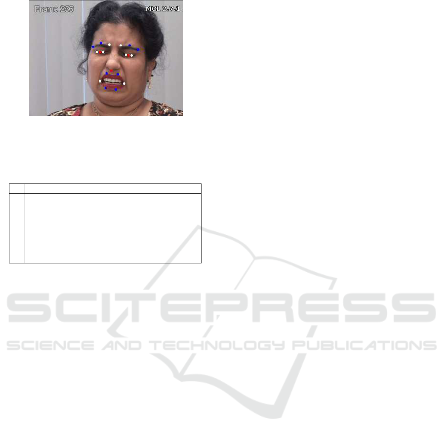
Figure 1: Sample in the UNBC-MSPEA database: A white

or red point represents a landmark for landmark-based fea-

tures and a white or blue point represents a landmark for

SIFTD.

Table 1: Pairs of landmarks for computing DFL.

# Pairs of landmarks

1 inner corners of right and left brows

2 right inner brow corner and nasal spine

3 left inner brow corner and nasal spine

4 right upper lid and lower lid

5 left upper lid and lower lid

6 right outer lid corner and right outer lip corner

7 left outer lid corner and left outer lip corner

25 patients performing a series of active and pas-

sive range-of-motion tests to their affected and un-

affected limbs. All images in this dataset were an-

notated by Active Appearance Model (AMM) land-

marks (Matthews and Baker, 2004) and the Prkachin

and Solomon pain intensity (PSPI) metric (Prkachin

and Solomon, 2008). A sample image and AAM

landmarks are shown in Fig. 1. We used images of

10 subjects who exposed high intensity painful facial

expressions (PSPI > 6). Low intensity painful facial

expression images (0 < PSPI ≤ 6) were not used. The

number of used images were 19,429 including 383

painful facial expression images.

4.2 Feature Extraction

Since OCSTM is a one-class method, the following

requirements for features are necessary: (1) normal

and anomalous samples in the target domain are sep-

arated in the feature space, (2) there are at least a few

source samples which are close to the target normal

samples. If (1) is not satisﬁed, the algorithm of OC-

STM gives large weights to the samples which are

close to the anomalous samples. If (2) is not satisﬁed,

all source samples are far from the target samples, and

the source samples do not help to predict the classes

of the target samples.

To investigate features suitable for the one-class

methods, we applied two ordinary appearance-based

extraction methods, Scale-Invariant Feature Trans-

form Descriptors (SIFTDs) (Sangineto et al., 2014)

and Local Binary Pattern Histograms feature (LBPH)

(Ahonen et al., 2006) as well as simple landmark-

based features, i.e., distances between pairs of land-

marks (Fig. 1). For detecting face and facial points in

the three feature extraction methods and for extracting

the landmark-based features, AMM landmarks anno-

tated to all images were employed.

SIFTD is a local feature, and is thus suitable for

anomalous facial expressions analysis. This is be-

cause an anomalous facial expression is related to

AUs which are localized to speciﬁc face regions.

Firstly the face was detected, aligned, and resized to a

200 × 200 pixel window. Then descriptors were com-

puted within 36 × 36 pixel regions around predeter-

mined 16 facial landmarks (Fig. 1). The length of the

descriptor is 128 for each region and thus the length

of the feature is 128 × 16 = 2,048 for each image.

LBPH is also a local feature and thus suitable

for anomalous facial expression analysis. Firstly, the

face was detected, aligned, and resized to a 128×128

pixel window. Then the resized face image was di-

vided to 8 × 8 blocks and the LBP histograms were

extracted from the blocks. We apply uni f orm LBP

8,1

to each block, where u2 means ”uniform”, and (8,1)

represents 8 sampling points on a circle of radius 1.

From each block, a 59-dimensional feature was ex-

tracted and thus the length of the LBP histogram is

59 × 8 × 8 = 3,776.

Face landmarks is one of the most applied fea-

tures for facial expression analyses. Typically, high-

dimensional features contain more noise than low-

dimensional ones. Thus we use simple features, i.e.,

landmark distances, which are related to painful fa-

cial expressions. In (Lucey et al., 2011), PSPI was

decided based on AUs, brow lowering (AU4), cheek

raising (AU6), eyelid tightening (AU7), nose wrin-

kling (AU9), upper-lip raising (AU10) and eye clos-

ing (AU 43). We selected seven distances related to

the AUs in Table 1. The distances were computed

based on normalized coordinates. Here x and y co-

ordinates are respectively normalized by the distance

between the inner corners of the eyes and the distance

between the middle of the eyes and the nasal spine

for each image. We refer to these Distances of Face

Landmarks as DFL and the length of the feature is 7.

4.3 Evaluation Protocol and Parameter

Setting

Since images in which a painful facial expression is

exposed are scarce (1.97%), we used them as anoma-

lous samples and normal samples as the rest. Follow-

ing other articles, experiments were conducted using

One-class Selective Transfer Machine for Personalized Anomalous Facial Expression Detection

279

Table 2: Comparison with relevant methods on DFL features (n

tar

= 500). Each row shows the result when the each subject

was used for the test subject and the last row shows their average.

F1 score AUC

subject

T-

OCSVM

ST-

OCSVM

ML-

OCSVM OCSTM

T-

OCSVM

ST-

OCSVM

ML-

OCSVM OCSTM

1 0.11 0.27 0.12 0.21 0.99 1.00 1.00 0.99

2 0.31 0 0.29 0.54 0.99 0.67 1.00 1.00

3 0.88 0.93 0.85 0.90 1.00 1.00 1.00 1.00

4 0.60 0 0.54 0.61 0.89 0.53 0.90 0.85

5 0 0 0 0 0.50 0.76 0.46 0.77

6 0.15 0.23 0.14 0.21 0.96 0.96 0.93 0.97

7 0.34 0.67 0.40 0.56 1.00 1.00 1.00 1.00

8 0.75 0.49 0.75 0.73 0.95 0.76 0.94 0.91

9 0.67 0 0.69 0.82 0.99 0.24 1.00 1.00

10 0 0 0 0 0.48 0.52 0.41 0.72

average 0.38 0.26 0.38 0.46 0.88 0.74 0.86 0.92

a leave-one-subject-out evaluation scheme in which

one subject in turn was chosen as the target and the

others as the source. Each image was treated inde-

pendently, i.e., no temporal information was used.

The n

tar

target samples were randomly selected from

the target subject, and the rest of the target samples

were used for the test. The Area Under the ROC

Curve (AUC) and F1 score were used for evaluation,

where F1 =

2·Precision·Recall

Precision+Recall

. We deﬁne F1 = 0 when

the number of anomalous samples which the classi-

ﬁer predicts as anomalous is zero

. We repeated the

experiments ﬁve times (except in Sec. 4.7 one time)

on each person for each method, and the averages of

AUC and F1 scores were reported.

We used Gaussian kernel with a bandwidth equal

to the mean distance between the target training sam-

ples. We set the parameter ν, which implies an up-

per bound on the fraction of anomaly samples on the

source and target samples, as ν = 0.0001 since we

used only normal samples for training OCSTM.

Furthermore, we set three parameters differently

from STM. Firstly, we set ε as follows. The ﬁrst and

second constraints in Eq. (7) together derive the fol-

lowing requirement for s, 1 ≤

νn

all

∑

all

i=1

. To ensure

this inequality through the second constraint in Eq.

(10), we set ε = 1 − νn

all

Secondly, we set the parameter B, i.e., the upper

bound of s

in Eq. (10), based on the ratio of the

source samples. In (Chu et al., 2013), B was set to

a large value. We observed that under such a set-

ting, only a small number of source samples tend to

be re-weighted largely, even if there are more source

samples which are close to target samples. There-

fore, we set B to the reciprocal of the ratio of the

source samples which are close to target samples, i.e.,

B = n

, where n

is the number of source sam-

ples whose average similarity measured by the Gaus-

In this case, Precision and Recall are both zero.

sian kernel function to the target samples is larger

than that between target samples. If n

= 0, we set

B = 10, 000 so that none of the s

reaches the upper

bound B, and in this case s

does not depend on B.

Thirdly, we scale the parameter λ by n

to balance

the slack variables ξ

ξ and κ

κ. In Eq. (10), the

λνn

all

tends to be signiﬁcantly smaller than κ

κ due to the term

all

. In addition, κ

κ is weighted by n

by deﬁnition,

i.e., κ

tar

∑

tar

j=1

k(x

tar

). Since n

and n

all

for

the target person are different from those of the other

persons, and n

is nearly equal to n

all

, we set λ as λ =

. In Sec. 4.7, we investigated the dependency of

OCSTM on the parameter λ

. Since the dependency

is small, we set λ

= 1,000 in all experiments except

in Sec. 4.7.

4.4 Comparison with Related Methods

In this section, we demonstrate the effectiveness of

OCSTM for anomalous facial expression detection

compared with related methods. Since we sup-

pose that only one-class samples are available, we

treat three one-class methods as compared methods,

i.e., OCSVM trained on the only target samples (T-

OCSVM), OCSVM trained on the source and target

samples (ST-OCSVM), and a state-of-the-art multi-

task learning with one-class SVM (ML-OCSVM) (He

et al., 2014). These methods were implemented by

us and the parameters for each method were tuned so

that it exhibits the best result. For this comparison,

we used DFL features.

Table 2 shows the F1 scores and AUC of the com-

pared methods. We see that our approach outperforms

In the empirical risk of STM, the training loss is

not weighted by n

all

, i.e., C

∑

i=1

), where n

means the number of the source samples in this paper,

(y,·) is a loss function for each sample whose class la-

bel is y, and C is a constant parameter.

VISAPP 2018 - International Conference on Computer Vision Theory and Applications

280

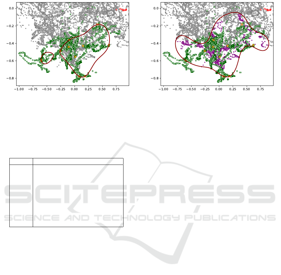
(a) T-OCSVM on target samples (b) OCSTM on target and source samples

Figure 2: 2D PCA projections of the samples and the hyperplanes for T-OCSVM and OCSTM when n

tar

= 10. Green and red

squares respectively represent normal and anomalous test samples in the target domain, and orange crosses and gray squares

respectively represent normal training samples in the target and source domains. A red closed surface represents a hyperplane

of each classiﬁer which predicts a sample inside as normal.

Table 3: Average similarities between the normal and

anomalous samples in the target domain, computed by the

Gaussian kernel function.

subject normal-anomalous normal-normal

1 0.140 0.331

2 0.019 0.358

3 0.007 0.345

4 0.256 0.372

5 0.411 0.333

6 0.012 0.316

7 0.003 0.361

8 0.169 0.321

9 0.178 0.406

10 0.418 0.362

all the other methods on average. The higher scores

of OCSTM compared with T-OCSVM are not sur-

prising because T-OCSVM was learnt from only lim-

ited training samples and thus suffered from overﬁt-

ting. As discussed in Sec. 1, ST-OCSVM cannot han-

dle the individual differences appropriately, resulting

in low F1 scores for several subjects. The scores

of ML-OCSVM are close to those of T-OCSVM.

This is because that ML-OCSVM combines the ST-

OCSVM and T-OCSVM models and a higher combi-

nation weight for T-OCSVM was selected. In contrast

to ML-OCSVM, which can only produce intermedi-

ate classiﬁers of two models, OCSTM ﬁts the target

distribution better since OCSTM selects source sam-

ples which are close to the target samples.

Table 3 shows the average similarities between the

normal and anomalous samples in the target domain,

and the similarity is given by the Gaussian kernel

function. For subjects #5 and #10, the similarity be-

tween the normal and anomalous samples in the target

domain is larger than that between the target normal

samples. Therefore, the requirement (1) in Sec. 4.2 is

violated, and F1 scores are zero (Table 2).

Fig. 2 shows 2D PCA projections of the samples

and the hyperplanes for T-OCSVM and OCSTM. In

Fig. 2, green and red squares respectively represent

the normal and anomalous test samples in the target

domain, and orange crosses and gray squares respec-

tively represent the normal training samples in the tar-

get and source domains. Purple squares in Fig. 2

(b) represent the source samples that are given larger

instance-wise weights than the mean. Since we used

non-linear feature mapping, a hyperplane is a closed

surface in the example space. A red closed surface

represents a hyperplane of each classiﬁer which pre-

dicts a sample inside as normal. In Fig. 2 (a) many

normal test samples are outside the closed surface,

which signiﬁes that the model of T-OCSVM overﬁts

to a few target samples. Conversely, in Fig. 2 (b) more

normal test samples are inside the closed surface than

T-OCSVM in Fig. 2 (a), which signiﬁes that OCSTM

avoids overﬁtting unlike T-OCSVM. Since in Eq. (2),

small weights s are given to the slack variables ξ

ξ of

the source samples which are far from the target sam-

ples, OCSTM hardly considers such samples. Con-

sequently, the optimization in Eq. (1) yields a hyper-

plane such that the target samples and the source sam-

ples which are close to the target samples are inside

the closed surface.

4.5 Comparison of Feature Extraction

Methods for OCSTM

In this section, we investigate the dependency of the

proposed method on the feature extraction methods.

As mentioned in Sec. 4.2, the two requirements for

features are necessary in OCSTM. We conducted ex-

periments using the three feature extraction methods.

One-class Selective Transfer Machine for Personalized Anomalous Facial Expression Detection

281

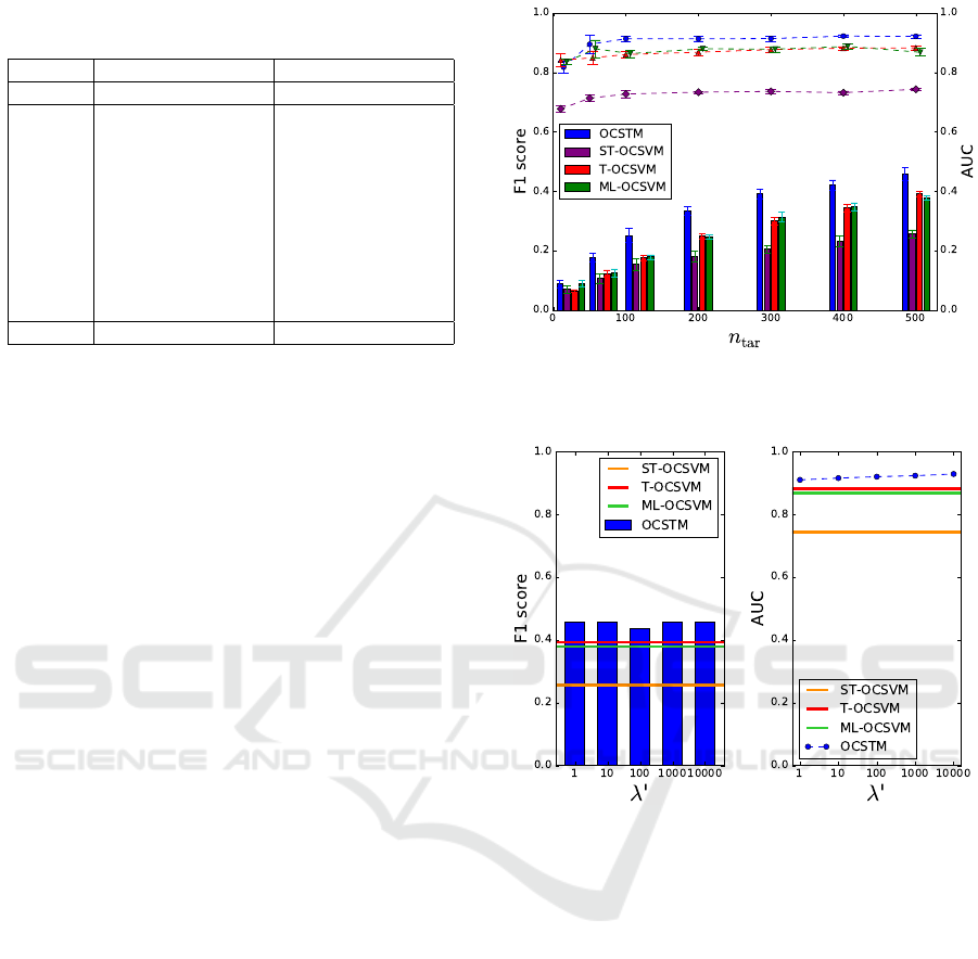
Table 4: F1 score using three feature extraction methods for

OCSVM and OCSTM (n

tar

= 500).

T-OCSVM OCSTM

subject LBPH SIFTD DFL LBPH SIFTD DFL

1 0.03 0.03 0.11 0.07 0.05 0.21

2 0.11 0.13 0.31 0.20 0.18 0.54

3 0.64 0.69 0.88 0.72 0.75 0.90

4 0.45 0.52 0.60 0.59 0.59 0.61

5 0.06 0.08 0 0.09 0.15 0

6 0.06 0.06 0.15 0.08 0.08 0.21

7 0.11 0.14 0.34 0.18 0.18 0.56

8 0.52 0.59 0.75 0.60 0.62 0.73

9 0.35 0.41 0.67 0.44 0.43 0.82

10 0.46 0.45 0 0.63 0.52 0

average 0.28 0.31 0.38 0.36 0.35 0.46

Table 4 shows F1 scores of T-OCSVM and OC-

STM using three kinds of features, LBPH, SIFTD and

DFL. The OCSTM outperforms T-OCSVM for each

feature extraction method in F1 score, and the results

show that the source samples which are close to the

target samples help to predict the classes of the test

samples accurately. Table 4 also shows that the F1

scores using DFL are higher than those using features

LBPH and SIFTD. This is because high-dimensional

features, i.e., LBPH and SIFTD, contain more irrele-

vant information than low-dimension ones, i.e., DFL.

As mentioned in Sec. 4.4, the F1 scores of OC-

STM with DFL features for subjects #5 and #10 are

zero because the similarity between the normal and

anomalous samples in the target domain is larger than

that between the target normal samples. On the other

hand, in OCSTM with LBPH and SIFTD features, we

conﬁrmed that the similarity between the normal and

anomalous samples in the target domain is smaller

than that between the target normal samples for all

subjects. Thus the requirement (1) in Sec. 4.2 is sat-

isﬁed and the F1 scores are not zero.

4.6 Performance Analysis in Terms of

the Number of the Target Samples

In this section, we analyze how the performance of

our method depends on the number of target samples

tar

. We conducted experiments using DFL by vary-

ing n

tar

from 10 to 500.

Fig. 3 shows the F1 scores and AUC of OCSTM

and the compared methods. We see that the perfor-

mance decreases as n

tar

decreases. OCSTM outper-

forms the other methods for each n

tar

in F1 score and

AUC, except for AUC when n

tar

= 10. The F1 score

of OCSTM when n

tar

= 300 is higher than those of the

other methods when n

tar

= 500. We can safely con-

clude that OCSTM avoids overﬁtting better than the

other methods.

Figure 3: Performance of OCSTM with respect to the num-

ber n

tar

of target samples. A line graph and a bar graph

respectively represent F1 scores and AUC for each method.

Figure 4: F1 scores and AUC of OCSTM with respect to

the parameter λ

tar

= 500). For comparison, the scores of

the other methods are shown as horizontal lines.

4.7 Dependency of OCSTM on the

Parameter λ

Here we analyze how the performance of our method

depends on the parameter λ = λ

. We con-

ducted experiments using DFL by varying λ

∈

{1,10,100,1000,10000} when n

tar

= 500.

Fig. 4 shows the F1 scores and AUC of OC-

STM with respect to parameter λ

and the scores of

the other compared methods. Note that scores of the

compared methods are the best scores by varying their

parameters. We see that the performance of OCSTM

does not largely depend on the parameter λ

. Al-

though when λ

= 100 the F1 score of OCSTM is

lowest, the performance is still higher than the other

methods.

VISAPP 2018 - International Conference on Computer Vision Theory and Applications

282

5 CONCLUSIONS

In this paper, we proposed a one-class transfer

learning method named OCSTM, for personalized

anomalous facial expression detection. Unlike other

anomaly detection methods, the OCSTM learns a per-

sonalized model from the target and source samples

by re-weighting the samples based on their proximity

to the target samples. Therefore, re-weighted sam-

ples help the target model to avoid overﬁtting even

if the sample size of the target samples is small, and

the classiﬁer handles the individual differences appro-

priately. Experiments conducted on UNBC-MSPEA

database show that OCSTM outperforms original

one-class SVM including the generic and single-task

model, and the state-of-the-art ML method. Further-

more, since the selection of feature extraction meth-

ods highly inﬂuences the performance of one-class

methods, we investigated suitable features for OC-

STM in anomalous facial expression detection. The

results show that DFL produces higher accuracies

than LBPH and SIFTD because low-dimension fea-

tures, i.e., DFL, contain less irrelevant information

than high-dimension ones, i.e., LBPH and SIFTD.

ACKNOWLEDGEMENTS

This work was partially supported by JSPS KAK-

ENHI Grant Number JP15K12100.

REFERENCES

Ahonen, T., Hadid, A., and Pietik

ainen, M. (2006). Face

Description with Local Binary Patterns: Applica-

tion to Face Recognition. IEEE Trans. on PAMI,

28(12):2037–2041.

Amari, S. and Wu, S. (1999). Improving Support Vector

Machine Classiﬁers by Modifying Kernel Functions.

Neural Networks, 12(6):783–789.

Chapelle, O. (2007). Training a Support Vector Machine in

the Primal. Neural Computation, 19(5):1155–1178.

Chen, J. and Liu, X. (2014). Transfer Learning with One-

Class Data. Pattern Recognition Letters, 37:32–40.

Chen, J., Liu, X., Tu, P., and Aragones, A. (2013). Learn-

ing Person-Speciﬁc Models for Facial Expression and

Action Unit Recognition. Pattern Recognition Letters,

34(15):1964–1970.

Chu, W.-S., Torre, F. D. L., and Cohn, J. F. (2013). Selective

Transfer Machine for Personalized Facial Action Unit

Detection. In CVPR, pages 3515–3522.

Ekman, P. and Friesen, W. V. (1978). Facial Action Coding

System. Consulting Psychologists Press, Palo Alto,

CA.

Gorski, J., Pfeuffer, F., and Klamroth, K. (2007). Bicon-

vex Sets and Optimization with Biconvex Functions:

a Survey and Extensions. Mathematical Methods of

Operations Research, 66(3):373–407.

Gretton, A., Smola, A., Huang, J., Schmittfull, M., Borg-

wardt, K., and Sch

olkopf, B. (2009). Covariate Shift

by Kernel Mean Matching, chapter 8, pages 131–160.

MIT Press, Cambridge, MA.

He, X., Mourot, G., Maquin, D., Ragot, J., Beauseroy,

P., Smolarz, A., and Grall-Ma

es, E. (2014). Multi-

Task Learning with One-Class SVM. Neurocomput-

ing, 133:416–426.

Lucey, P., Cohn, J. F., Prkachin, K. M., Solomon,

P. E., and Matthews, I. (2011). Painful Data: The

UNBC-McMaster Shoulder Pain Expression Archive

Database. In FG, pages 57–64.

Matthews, I. and Baker, S. (2004). Active Appearance

Models Revisited. International Journal of Computer

Vision, 60(2):135–164.

Mohammadian, A., Aghaeinia, H., Towhidkhah, F., et al.

(2016). Subject Adaptation Using Selective Style

Transfer Mapping for Detection of Facial Action

Units. Expert Systems with Applications, 56:282–290.

Prkachin, K. M. and Solomon, P. E. (2008). The Structure,

Reliability and Validity of Pain Expression: Evidence

from Patients with Shoulder Pain. Pain, 139(2):267–

274.

Sangineto, E., Zen, G., Ricci, E., and Sebe, N. (2014). We

are not All Equal: Personalizing Models for Facial Ex-

pression Analysis with Transductive Parameter Trans-

fer. In ACM Multimedia, pages 357–366.

Sch

olkopf, B., Platt, J. C., Shawe-Taylor, J., Smola, A. J.,

and Williamson, R. C. (2001). Estimating the Support

of a High-Dimensional Distribution. Neural Compu-

tation, 13(7):1443–1471.

Shan, C., Gong, S., and McOwan, P. W. (2009). Facial Ex-

pression Recognition Based on Local Binary Patterns:

A Comprehensive Study. Image and Vision Comput-

ing, 27(6):803–816.

Zen, G., Porzi, L., Sangineto, E., Ricci, E., and Sebe, N.

(2016). Learning Personalized Models for Facial Ex-

pression Analysis and Gesture Recognition. IEEE

Trans. on Multimedia, 18(4):775–788.

Zeng, J., Chu, W.-S., Torre, F. D. L., Cohn, J. F., and Xiong,

Z. (2015). Conﬁdence Preserving Machine for Facial

Action Unit Detection. In ICCV, pages 3622–3630.

Zeng, Z., Fu, Y., Roisman, G. I., Wen, Z., Hu, Y., and

Huang, T. S. (2006). One-Class Classiﬁcation for

Spontaneous Facial Expression Analysis. In FG,

pages 281–286.

Zeng, Z., Pantic, M., Roisman, G. I., and Huang, T. S.

(2009). A Survey of Affect Recognition Methods:

Audio, Visual, and Spontaneous Expressions. IEEE

Trans. on PAMI, 31(1):39–58.

One-class Selective Transfer Machine for Personalized Anomalous Facial Expression Detection

283