A Model-checking Approach to Reduce Spiking Neural Networks

Elisabetta De Maria

, Daniel Gaff

, C

edric Girard Riboulleau

and Annie Ressouche

Univ. C

ote d’Azur, CNRS, I3S, UMR 7271, 06900 Sophia Antipolis, France

Univ. C

ote d’Azur, CNRS, LEAT, UMR 7248, 06900 Sophia Antipolis, France

Univ. C

ote d’Azur, INRIA SAM, 06902 Sophia-Antipolis, France

Keywords:

Neural Spiking Networks, Probabilistic Models, Temporal Logic, Model Checking, Network Reduction.

Abstract:

In this paper we formalize Boolean Probabilistic Leaky Integrate and Fire Neural Networks as Discrete-Time

Markov Chains using the language PRISM. In our models, the probability for neurons to emit spikes is driven

by the difference between their membrane potential and their ﬁring threshold. The potential value of each

neuron is computed taking into account both the current input signals and the past potential value. Taking

advantage of this modeling, we propose a novel algorithm which aims at reducing the number of neurons and

synaptical connections of a given network. The reduction preserves the desired dynamical behavior of the

network, which is formalized by means of temporal logic formulas and veriﬁed thanks to the PRISM model

checker.

1 INTRODUCTION

Since a few decades, neurobiologists and bioinfor-

matics researchers work in concert to model neural

networks, aiming at understanding the interactions

among neurons, and the way they participate in the

different vital functions of human beings. Models be-

come bigger and bigger, and the necessity of reduc-

ing them while preserving their expected dynamics

emerges, especially in the scope of the obtention of

models which are suitable for formal veriﬁcation. In

this paper we tackle the issue of neural network re-

duction.

In the literature neural network modeling is of-

ten classiﬁed into three generations (Maass, 1997;

Paugam-Moisy and Bohte, 2012). First generation

models, represented by McCulloch-Pitts one (McCul-

loch and Pitts, 1943), deal with discrete inputs and

outputs and their computational units are a set of

logic gates with a threshold activation function. Sec-

ond generation models, whose most known one is the

multi-layer perceptron (Cybenko, 1989), exploit real

valued activation functions. These networks, whose

real-valued outputs represent neuron ﬁring rates, are

extensively used in the domain of artiﬁcial intelli-

gence and are also known as artiﬁcial neural net-

works. Third generation networks, also called Spiking

Neural Networks (Paugam-Moisy and Bohte, 2012),

stand out for the relevance of time aspects. Precise

spike ﬁring times are taken into account. Further-

more, they consider not only current input spikes but

also past ones. In (Izhikevich, 2004), Spiking Neural

Networks are classiﬁed with respect to their biophys-

ical plausibility, that is, to the number of behaviors

(i.e., typical responses to an input pattern) they can

display. Among these models, the Hodgkin-Huxley

model (Hodgkin and Huxley, 1952) is the one able

to reproduce most behaviors. However, its simulation

process is really expensive even for a few neurons.

In this work we choose to rely on the Leaky In-

tegrate and Fire (LI&F) model (Lapicque, 1907), a

computationally efﬁcient approximation of a single-

compartment model. Our LI&F model is augmented

with probabilities. More precisely, the probability

for neurons to emit spikes is driven by the differ-

ence between their membrane potential and their ﬁr-

ing threshold. Probabilistic neurons are encoded as

Discrete-Time Markov Chains thanks to the model-

ing language at PRISM user’s disposition. PRISM

(Kwiatkowska et al., 2011) is a tool that allows not

only to model different probabilistic systems (with

discrete or continuous time, with or without nondeter-

minism), but also to specify their expected behavior

thanks to the use of temporal logics, a formalism for

describing the dynamical evolution of systems. Fur-

thermore, PRISM provides a model checker (Clarke

et al., 1999), which is a tool for automatically verify-

ing whether a given system satisﬁes or not a property

Maria, E., Gaffé, D., Riboulleau, C. and Ressouche, A.

A Model-checking Approach to Reduce Spiking Neural Networks.

DOI: 10.5220/0006572000890096

In Proceedings of the 11th International Joint Conference on Biomedical Engineering Systems and Technologies (BIOSTEC 2018) - Volume 3: BIOINFORMATICS, pages 89-96

ISBN: 978-989-758-280-6

expressed in temporal logic. In case the property does

not hold in the system, the user can have access to a

counter-example, that is, an execution trace falsify-

ing the property at issue, which often helps in ﬁnding

modiﬁcations in the model for the property to be sat-

isﬁed. In order to apply model-checking techniques

efﬁciently, the model to handle should be as small as

possible.

Taking advantage of this modeling and veriﬁ-

cation framework, we introduce a novel algorithm

which aims at reducing the number of neurons and

synaptical connections of a given neural network.

The proposed reduction preserves the desired dynam-

ical behavior of the network, which is formalized by

means of temporal logic formulas and veriﬁed thanks

to the PRISM model checker. More precisely, a neu-

ron is removed if its suppression has a low impact on

the probability for a given temporal logic formula to

hold. Observe that, other than their utility in lighten-

ing models, algorithms for neural network reduction

have a forthright application in the medical domain.

In fact, they can help in detecting weakly active (or

inactive) zones of the human brain.

The issue of reducing biological networks is not

new in systems biology. Emblematic examples can

be found in (Naldi et al., 2011), where the authors

propose a methodology to reduce regulatory networks

preserving some dynamical properties of the original

models, such as stable states, in (Gay et al., 2010),

where the authors study model reductions as graph

matching problems, or in (Paulev

e, 2016), whose au-

thor considers ﬁnite-state machines and proposes a

technique to remove some transitions while preserv-

ing all the (minimal) traces satisfying a given reach-

ability property. As far as neural networks are con-

cerned, to the best of our knowledge the core of the

existing reduction approaches only deals with second

generation networks. Several methods to train a net-

work that is larger than necessary and then remove

the superﬂuous parts, known as pruning techniques,

are explained in (Reed, 1993) . Finally, in (Menke

and Martinez, 2009) the authors introduce an ora-

cle learning methodology, which consists in using a

larger model as an oracle to train a smaller model in

order to obtain a smaller acceptable model. With ora-

cle learning, the smaller model is created initially and

trained using the larger model, whereas with pruning,

connections are removed from the larger model until

the desired size is reached.

The paper is organized as follows. In Section 2

we introduce a probabilistic version of the Leaky In-

tegrate and Fire Model. Section 3 is devoted to the

PRISM modeling language and the temporal logic

PCTL (Probabilistic Computation Tree Logic). In

Section 4 we describe our modeling of neural net-

works as Discrete-Time Markov Chains in PRISM.

2 PROBABILISTIC LEAKY

INTEGRATE AND FIRE

MODEL

We model neuron networks as Boolean Spiking Net-

works, where the electrical properties of neurons

are represented through the Leaky Integrate and Fire

(LI&F) model. In this modeling framework, neural

networks are seen as directed graphs whose nodes

stand for neurons and whose edges stand for synap-

tical connections. Edges are decorated with weights:

positive (resp. negative) weights represent activations

(resp. inhibitions). The dynamics of each neuron is

characterized through its (membrane) potential value,

which represents the difference of electrical potential

across the cell membrane. At each time unit, the po-

tential value is computed taking into account present

input spikes and the previous decayed potential value.

In order to weaken the past potential value, it is mul-

tiplied by a leak factor. In our probabilistic LI&F

model, the probability for each neuron to emit an ac-

tion potential, or spike, is governed by the difference

between the potential value and a given ﬁring thresh-

old. For positive (resp. negative) values of this dif-

ference, the more its absolute value is big, the more

(resp. the less) is the probability to emit a spike. Af-

ter each spike emission, the neuron potential is reset

to zero. In the literature, other ways exist to incorpo-

rate probabilities in LI&F models, such as the Noisy

Integrate and Fire models (Di Maio et al., 2004; Four-

caud and Brunel, 2002), where a noise is added to the

computation of the potential value.

More formally, we give the following deﬁnitions

for probabilistic LI&F networks.

Deﬁnition 1 (Boolean Probabilistic Spiking Integrate

and Fire Neural Network). A Boolean Probabilis-

tic Integrate and Fire Neural Network is a tuple

(V, E, w), where:

• V are Boolean probabilistic spiking integrate and

ﬁre neurons,

• E ⊆ V ×V are synapses,

• w : E → Q ∩[−1, 1] is the synapse weight function

associating to each synapse (u, v) a weight w

We distinguish three disjoint sets of neurons: V

(input

neurons), V

int

(intermediary neurons), and V

(output

neurons), with V = V

∪V

int

∪V

Deﬁnition 2 (Boolean Probabilistic Spiking Integrate

and Fire Neuron). A Boolean Probabilistic Spiking

BIOINFORMATICS 2018 - 9th International Conference on Bioinformatics Models, Methods and Algorithms

Integrate and Fire Neuron v is a tuple (τ, r, p, y),

where:

• τ ∈ N is the ﬁring threshold,

• r ∈ Q ∩ [0, 1] is the leak factor,

• p : N → Q

is the [membrane] potential function

deﬁned as

p(t) =



∑

i=1

· x

(t), i f p(t − 1) > τ

∑

i=1

· x

(t) + r · p(t − 1), otherwise

where p(0) = 0, m is the number of inputs of the

neuron v, w

is the weight of the synapse connect-

ing the i

input neuron of v to the neuron v, and

(t) ∈ {0, 1} is the signal received at the time t by

the neuron v through its i

input synapse (observe

that, after the potential overcomes its threshold, it

is reset to 0),

• y : N → {0, 1} is the output function of the neuron.

Supposing to discretize p(t) − τ in k + 1 positive in-

tervals and k + 1 negative intervals, the probability

for the neuron v to emit a spike can be described as

follows:

P(y(t) = 1) =











1 i f p(t)− τ ≥ l

i f l

k−1

≤ p(t) − τ < l

k+1

i f 0 ≤ p(t) − τ < l

i f − l

≤ p(t) − τ < 0

i f − l

≤ p(t) − τ < −l

k−1

0 i f p(t)− τ < −l

(1)

with {l

, .. . , l

} ⊆ N

such that l

< l

i+1

∀i ∈

{1, .. . , k − 1} and {p

, .. . , p

} ⊆ ]0, 1] ∩Q such that

< p

i+1

∀i ∈ {1, . . . , 2k − 1}.

In our implementation, the probability values are cho-

sen in order to conform to a sigmoidal function.

3 THE PROBABILISTIC MODEL

CHECKER PRISM

The probabilistic model checker PRISM

(Kwiatkowska et al., 2011) is a tool for formal

modeling and analysis of systems with a random or

probabilistic behavior. It supports several types of

probabilistic models: discrete ones, namely discrete-

time Markov chains, Markov decision processes, and

probabilistic automata, and continuous ones, namely

continuous-time Markov chains, probabilistic timed

automata, and priced probabilistic timed automata.

In this work we rely on discrete-time Markov chains,

which are transition systems augmented with prob-

abilities. Their set of states represent the possible

conﬁgurations of the system being modeled, and

transitions between states model the evolution of

the system, which occurs in discrete-time steps.

Probabilities of making transitions between states are

given by discrete probability distributions. Markov

chains are memoryless, that is, their current state

contains all the information needed to compute

future states (Markov property). More precisely, the

following deﬁnition can be given:

Deﬁnition 3 (Discrete-Time Markov Chain). A

Discrete-Time Markov Chain (DTMC) over a set of

atomic propositions AP is a tuple (S, S

init

, P, L) where:

• S is a set of states (state space)

• S

init

⊆ S is the set of initial states

• P : S × S → [0, 1] is the transition probability ma-

trix, where

∑

∈S

P(s, s

) = 1 for all s ∈ S

• L : S → 2

is a function labeling states with

atomic propositions over AP.

An example of DTMC representing a simpliﬁed

neuron is graphically depicted in Figure 1, where the

neuron can be either active or inactive.

Figure 1: Example of a two-state DTMC representing a

simpliﬁed neuron. When the neuron is inactive (state 0), it

remains inactive with a probability of 0.5, and it becomes

active, and thus emits a spike (state 1), with a probability of

0.5. When it is active, is becomes inactive with a probability

of 1.

3.1 The PRISM Modeling Language

PRISM provides a state-based modeling language in-

spired from the reactive modules formalism of (Alur

and Henzinger, 1999). A model is composed by a

set of modules which can interact with each other. At

each moment, the state of each module is given by the

values of its local variables, and the global state of the

whole model is determined by the local state of all its

modules. The dynamics of each module is described

by a set of commands of the form:

[]guard → prob

: update

+ ... + prob

: update

;

where guard is a predicate over all the variables of the

model, indicating the condition to be veriﬁed in order

to execute the command, and each update indicates

a possible transitions of the model, to be achieved

by giving new values to the variables of the module.

Each update is assigned to a probability and, for each

A Model-checking Approach to Reduce Spiking Neural Networks

command, the sum of probabilities must be 1. The

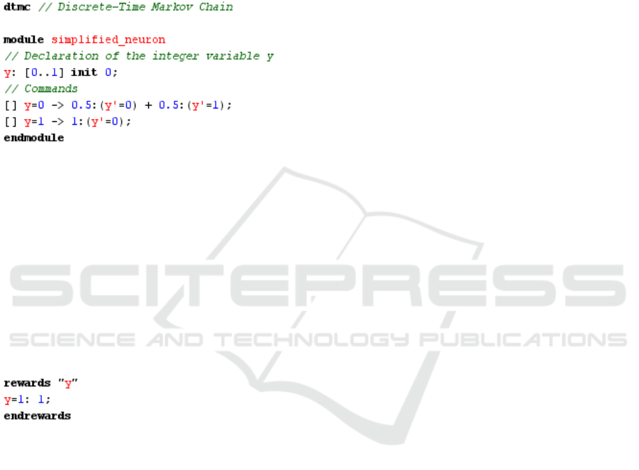
PRISM code for the DTMC of Figure 1 is given in

Figure 2. In such a simple module, the square brack-

ets at the beginning of each command are empty but

it is possible to add labels representing actions. These

actions can be used to force two or more modules

to make transitions simultaneously. In this work, we

take advantage of this feature to synchronize neurons

in networks. Finally, PRISM models can be extended

Figure 2: PRISM code for the DTMC of Figure 1. The

only variable y, representing the state of the neuron, ranges

over [0..1]. Its initial value is 0. When the guard is y = 0,

the updates (y

= 0) and (y

= 1) and their associated proba-

bilities state that the value of y remains at 0 with probability

0.5 and passes to 1 with probability 0.5. When y = 1, the

variable changes its value to 0 with a probability of 1.

with rewards (Kwiatkowska et al., 2007), which al-

low to associate real values to states or transitions of

models. As an example, in Figure 3 we show how to

augment the simpliﬁed neuron code of Figure 2 in or-

der to add a reward each time the neuron is active, and

thus to count the number of spike emissions.

Figure 3: Addition of a reward to the PRISM code for a

simpliﬁed neuron. Each time y = 1 (spike emission), the

reward increases of one time unit.

3.2 Probabilistic Temporal Logic

PRISM allows to specify the dynamics of DTMCs

thanks to the temporal logic PCTL (Probabilistic

Computation Tree Logic) introduced in (Hansson and

Jonsson, 1994), which extends the logic CTL (Com-

putation Tree Logic) (Clarke et al., 1986) with time

and probabilities. The following state quantiﬁers are

available in PCTL: X (next time), which speciﬁes that

a property holds at the next state of a given path,

F (sometimes in the future), which requires a prop-

erty to hold at some state on the path, G (always in

the future), which imposes that a property is true at

every state on the path, and U (until), which holds

if there is a state on the path where the second of

its argument properties holds and, at every preced-

ing state on the path, the ﬁrst of its two argument

properties holds. Note that the classical path quan-

tiﬁers A (forall) and E (exist) of CTL are replaced

by probabilities. Thus, instead of saying that some

property holds for all paths or for some paths, we

can express that a property holds for a certain frac-

tion of the paths (Hansson and Jonsson, 1994). The

most important operator in PCTL is P, which al-

lows to reason about the probability of event occur-

rences. The property P bound [prop] is true in a

state s of a model if the probability that the prop-

erty prop is satisﬁed by the paths from state s sat-

isﬁes the bound bound. As an example, the PCTL

property P= 0.5 [X (y = 1)] holds in a state if the

probability that y = 1 is true in the next state equals

0.5. All the state quantiﬁers given above, with the

exception of X, have bounded variants, where a time

bound is imposed on the property. For example, the

property P> 0.9 [F<=10 y=1] is true in a state if the

probability of y being equal to 1 within 10 time units

is greater than 0.9. Furthermore, in order to com-

pute the actual probability that some behavior of a

model is displayed, the P operator can take the form

P=? [prop], which evaluates to a numerical rather

than to a Boolean value. As an example, the property

P =? [G (y = 0)] expresses the probability that y

is always equal to 0.

PRISM also allows to formalize properties which

relate to the expected values of rewards. This is pos-

sible thanks to the R operator, which can be used in

the following two forms: R bound [rewardprop],

which is true in a state of a model if the expected re-

ward associated with reward prop when starting from

that state meets the bound, and R=? [rewardprop],

which returns the actual expected reward value. Some

speciﬁc operators are introduced in PRISM in order

to deal with rewards. In the rest of the paper, we

mainly exploit C (cumulative-reward). The property

C<=t corresponds to the reward cumulated along a

path until t time units have elapsed. As an exam-

ple, consider the reward y of Figure 3. The property

R{"y"} =? [C <= 100] returns the expected value

of the reward y within 100 time units. PRISM pro-

vides model-checking algorithms (Clarke et al., 1999)

to automatically validate DTMCs over PCTL proper-

ties and reward-based ones. The available algorithms

are able to compute the actual probability that some

behavior of a model is displayed, when required.

BIOINFORMATICS 2018 - 9th International Conference on Bioinformatics Models, Methods and Algorithms

4 NEURONAL NETWORKS IN

PRISM

This section is devoted to the modeling of Boolean

Probabilistic LI&F neural networks as DTMCs using

the PRISM language. As a ﬁrst step, we introduce

an input generator module in order to generate input

sequences on the alphabet {0, 1} for input neurons.

Such a module deals with one only Boolean variable

whose value is 1 (resp. 0) in case of spike (resp. no

spike) emission. We provide several instantiations of

such a module to be able to generate different kinds

of input sequences: persistent ones (containing only

1), oscillatory ones, and random ones.

We then deﬁne a neuron module to encode LI&F

neurons. The state of each neuron is characterized by

two variables: a ﬁrst Boolean variable denoting the

spike emission, and a second integer

variable repre-

senting the potential value, computed as a function of

the current inputs and the previous potential value, as

shown in Deﬁnition 2. The difference between the

potential value and the ﬁring threshold is discretized

into k + 1 positive intervals and k + 1 negative inter-

vals and a PRISM command is associated to each one

of this intervals: if the neuron is inactive and the dif-

ference between the potential and the threshold meets

the guard, the neuron is activated with a certain prob-

ability p (a bigger difference gives a higher probabil-

ity). The neuron remains inactive with a probability

equal to 1 − p. The aforecited commands share the

same label (to). To complete the modeling of a single

neuron, we add a command acting when the neuron is

active: with a probability of 1 it resets the potential

value and makes the neuron inactive. Such a com-

mand is connoted by a new different label (reset),

that turns out to be useful to synchronize the output of

neurons with the input of the following ones. Thanks

to a module renaming feature at PRISM user’s dispo-

sition, neurons with different parameters can be easily

obtained starting from the standard neuron module.

We then model the synaptical connections be-

tween the neurons of the network. In order to avoid a

neuron to be reset before its successor takes its acti-

vation into account, we introduce a transfer module

consisting of one only variable ranging over {0,1}

and being initialized at 0. Thanks to synchronization

labels, at each reset of the ﬁrst neuron this variable

passes to 1 ﬁrst, and then goes back to 0, synchroniz-

ing with the second neuron (label to), which takes the

received signal into account to compute its potential

value.

The PRISM code for the neuron and the transfer

We exploit integer rather than rational numbers in order to

have efﬁcient model-checking performances

modules can be found in (Girard Riboulleau, 2017),

where the PRISM model has been validated against

several PCTL properties.

5 MODEL-CHECKING BASED

REDUCTION ALGORITHM

In this section we introduce a novel algorithm for the

reduction of Boolean Probabilistic LI&F networks.

The algorithm supposes the network to be imple-

mented as a DTMC in PRISM (Girard Riboulleau,

2017) and makes several calls to the PRISM model

checker, in order to retrieve the probability relative to

the satisfaction of some PCTL formulas and the value

of some rewards.

As a ﬁrst step, the algorithm aims at identify-

ing, and thus removing, the wall neurons, that is, the

neurons that are not able emit, even if they receive

a persistent sequence of spikes as input. More for-

mally, a neuron can be characterized as a wall one if

its probability to be always quiescent (inactive) is 1:

P=1 [G (y=0)]. When the algorithm detects a wall

neuron, it removes not only the neuron but also its

descendants whose only incoming synaptical connec-

tion comes, directly or indirectly

, from this neuron,

and its ancestors whose only outgoing edge enters, di-

rectly or indirectly, the neuron.

As a second step, the algorithm aims at testing

whether the suppression of the remaining neurons

preserves or not the dynamics of the network. The

removal of a neuron (and its associated ancestors and

descendants) is authorized if the following two quan-

tities are kept (modulo a certain error):

Quantitative Criterion. The reward computing the

number of emitted spikes (within 100 time units)

of each output neuron.

Qualitative Criterion. The probability for a given

PCTL property (concerning the output neurons)

to hold.

The number of spikes emitted by a neuron

within 100 time units can be computed thanks

to the following reward-based PRISM property:

R{"y"} =? [C <= 100]. An example of key

property concerning the qualitative behavior of a

neuron is the following one, expressing an oscil-

lating trend: P=? [G((y=1 => (y=1 U y=0))&

(y=0 => (y=0 U y=1)))]. Such a formula requires

every spike emission to be followed by a quiescent

state (not necessarily immediately) and viceversa.

Formulas comparing the behaviors of several neurons

By one only edge or a path

A Model-checking Approach to Reduce Spiking Neural Networks

can be written as well. Observe that the respect of

both quantitative and qualitative criteria is needed for

a neuron removal. In fact, the output neurons of two

different networks could exhibit the same spike rate

but display a completely different behavior. On the

other hand, their could exhibit the same qualitative

behavior (e.g., an oscillatory trend), but have quite

different spike rates. The pseudo-code for the pro-

posed reduction algorithm is given in Algorithm 1. It

takes as input a Boolean Probabilistic LI&F network

G = (V, E, w) as given in Deﬁnition 1, a PCTL prop-

erty Prop concerning the dynamical behavior of the

output neurons of the network, and an allowed error

value ε. Only intermediary neurons are affected by

the reduction process, that is, input and output neu-

rons cannot be removed. Intermediary neurons are

ﬁrst visited following a depth ﬁrst search (DFS) in

order to remove wall neurones (and their associated

ancestors and descendants). We opt for a depth ﬁrst

visit instead of a breath ﬁrst visit to avoid expensive

backtracking. Furthermore, DFS is better suited to

our approach because it allows to quickly take into

account all the descendants of a node and cut them

if necessary. The procedure in charge to remove a

neuron (and its associated ancestors and descendants)

is REMOVAL (see Algorithm 2). Another depth ﬁrst

traversal of the (remaining) intermediary neurons is

then performed to identify (and thus remove thanks

to the REMOVAL procedure) neurons whose removal

has a low inﬂuence (according to ε) on the probabil-

ity for Prop to be satisﬁed and on the rate spike. It

is possible to see that, for each traversal, each edge

is visited at most twice, once forward and once back-

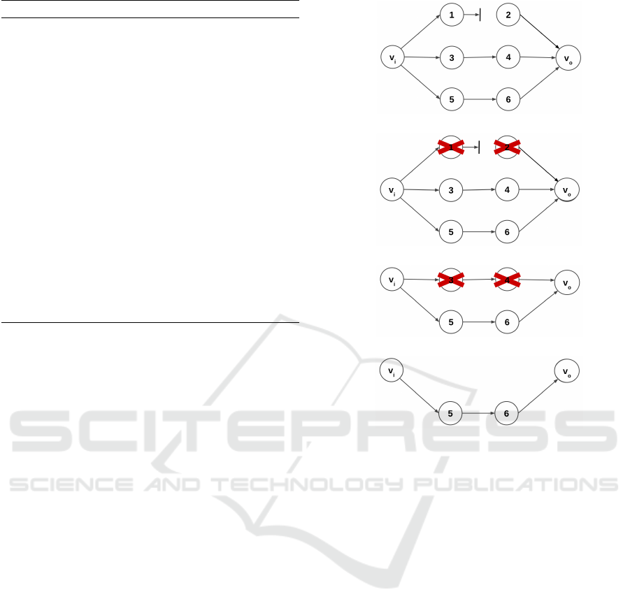
ward. An example of application of the algorithm to a

neural network composed of eight neurons and nine

edges is graphically depicted in Figure 4. The re-

duction process leads to a reduced network consisting

of four neurons and three edges. In Table 1 we con-

sider several neural networks composed of four neu-

rons (with only one input and output neuron) and their

corresponding reduced network, consisting of three

neurons. For each network, we give the spike rate of

the output neuron, and the number of states and transi-

tions of the corresponding PRISM transition system.

For an average error lower than 0.65 in the spike rate,

we have an average reduction of the state number of

a factor 19.6 and an average reduction of the transi-

tion number of a factor 19.64 when passing from the

complete to the reduced network.

Algorithm 1: LI&F REDUCTION (G, Prop, ε).

1: $$We distinguish input, intermediary, and output

neurons

2: Let V = V

int

3: for all v

∈ V

int

in a DFS visit do

4: Set to 1 all the input signals of v

5: $$ Call to the PRISM model checker

6: if P = 1[G(y

= 0)] $$ y

is the output of v

then

7: REMOVAL(v

) $$ V

int

and E are modiﬁed

by REMOVAL

8: Set to 1 all the input signals of the neurons of V

9: for all v

∈ V

10: Compute r

= spike rate o f v

thanks to

PRISM rewards

11: Compute p = Prob(Prop is T RU E) thanks to

PRISM

12: for all v

∈ V

int

13: Let V

= V \{v

}, E

= E \ {(v

, v

)∪ (v

, v

)}

s.t. v

, v

∈ V

14: Let G

= (V

, E

, w)

15: for all v

∈ V

16: Compute r

= spike rate o f v

in G

thanks to PRISM rewards

17: Compute p

= Prob(Prop is T RUE) in G

thanks to PRISM

18: if |r

− r

| ≤ ε for all v

∈ V

and |p

− p| ≤ ε

then

19: REMOVAL(v

)

Table 1: Comparative table of some complete and re-

duced networks. We consider 13 different (with differ-

ent parameters) networks composed of four neurons and the

corresponding networks obtained thanks to the reduction al-

gorithm. All the reduced networks consist of three neurons.

We give spike rates of output neurons, and the number of

states and transitions of the corresponding PRISM transi-

tion systems. The last row refers to averages.

Complete network (4 neurons) Reduced network (3 neurons)

spikes states transitions spikes states transitions

6.75 252 820 565 068 6.72 16 816 37 510

7.93 148 480 319 549 7.92 10 255 22 029

6.11 291 002 653 121 6.07 19 903 44 559

9.55 280 719 608 641 9.54 12 062 26 109

6.75 225 169 500 245 6.72 15 005 33 254

5.86 265 683 591 546 5.48 19 571 43 542

8.75 149 641 325 890 8.65 9 418 20 466

7.39 193 897 425 447 7.37 12 951 28 341

8.16 961 701 2 142 739 8.16 21 829 48 547

5.84 60 422 129 583 5.84 7 239 15 516

9.50 196 433 427 391 9.50 12 768 27 762

10.26 333 952 715 179 10.26 10 841 23 101

8.13 192 456 424 269 8.13 12 634 27 809

7.77 273 260 602 205 7.72 13 946 30 657

BIOINFORMATICS 2018 - 9th International Conference on Bioinformatics Models, Methods and Algorithms

Algorithm 2: REMOVAL(v

1: $$ It suppresses a neuron v

and all the neurons

only having v

as ancestor or descendant

2: V

int

= V

int

\ {v

}

3: E = E \ {(v

, v

) ∪ (v

, v

)} s.t. v

, v

∈ V

4: G

work

= (V

int

, E)

5: for all v

descendant of v

in a DFS visit of G do

6: $$ If v

has no incoming edges in G

work

, we

remove v

and its exiting edges

7: if {(v

, v

)} = ∅ then

8: V

int

= V

int

\ {v

}

9: E = E \{(v

, v

)} s.t. v

∈ V

10: for all v

ancestors of v

in a DFS visit of G do

11: $$ If v

has no outgoing edges in G

work

, we

remove v

and its incoming edges

12: if {(v

, v

)} = ∅ then

13: V

int

= V

int

\ {v

}

14: E = E \{(v

, v

)} s.t. v

∈ V

15: G = G

work

6 CONCLUSIONS

In this paper we have formalized Boolean Proba-

bilistic Leaky Integrate and Fire Neural Networks

as Discrete-Time Markov Chains using the language

PRISM. Taking advantage of this modeling, we have

proposed a novel algorithm which aims at reducing

the number of neurons and synaptical connections of

a given network. The reduction preserves the desired

dynamical behavior of the output neurons of the net-

work, which is formalized by means of temporal logic

formulas and veriﬁed thanks to the PRISM model

checker.

This work is the starting point for several future

research directions. From a modeling point of view,

the use of labels entails a break time during which the

different modules communicate but all the other func-

tions are stopped. Namely, in our model the reset

label causes a break time after each spike emission.

A big number of spikes leads thus to a big number of

break times and we intend to minimize these times.

We also plan to model the refractory time of neurons,

a lapse of time following the spike emission during

which the neuron is not able to emit (even if it con-

tinues to receive signals). At this aim, we may need

to take advantage of Probabilistic Timed Automata,

which are at PRISM user’s disposition.

Concerning the reduction algorithm, for the mo-

ment we show our approach to be efﬁcient for small

networks, i.e., the removal of only one neuron drasti-

cally reduces the size of the transition system. As for

future work, we intend to scale our methodology.

(a) Initial network

(b) First reduction

(d) Reduced network

Figure 4: Application of the reduction algorithm on a

neuronal network of eight neurons. The only input neu-

ron is v

and the only output neuron is v

. The other neurons

are numbered according to a DFS order. The neuron 1 is

identiﬁed as a wall one. The ﬁrst reduction step (4(b)) con-

sists in removing the neuron 1 and, consequently, the neu-

ron 2, because its only ingoing edge comes from the neuron

1. No other wall neuron is detected. The second reduction

(4(c)) is due to the fact that the removal of neuron 4 inﬂu-

ences neither the satisfaction of Prop nor the spike emission

rate of v

. The neuron 3 is also removed because its only

output edge enters the neuron 4. The ﬁnal reduced network

is given in 4(d).

The actual version of the reduction algorithm ﬁnds

a reduction which conforms to the expected behavior

of the network. We ﬁnd one solution among several

possible ones, but this solution is not necessary the

optimal one, that is, it does not necessarily minimize

the difference of behavior between the complete and

the reduced network. In order to help the research

of optimal solutions, we intend to perform a sensitiv-

ity analysis of our networks, aiming at identifying the

parameters playing a most important role in the veri-

ﬁcation of some given temporal properties.

A Model-checking Approach to Reduce Spiking Neural Networks

ACKNOWLEDGEMENTS

We thank Alexandre Muzy for fruitful discussions on

neuron behaviors.

REFERENCES

Alur, R. and Henzinger, T. (1999). Reactive modules. For-

mal Methods in System Design, 15(1):7–48.

Clarke, E. M., Emerson, E. A., and Sistla, A. P. (1986).

Automatic veriﬁcation of ﬁnite-state concurrent sys-

tems using temporal logic speciﬁcations. ACM Trans-

actions on Programming Languages and Systems

(TOPLAS), 8(2):244–263.

Clarke, E. M., Grumberg, O., and Peled, D. (1999). Model

checking. MIT press.

Cybenko, G. (1989). Approximation by superpositions of a

sigmoidal function. Mathematics of Control, Signals

and Systems, 2(4):303–314.

Di Maio, V., Lansky, P., and Rodriguez, R. (2004). Dif-

ferent types of noise in leaky integrate-and-ﬁre model

of neuronal dynamics with discrete periodical input.

General physiology and biophysics, 23:21–38.

Fourcaud, N. and Brunel, N. (2002). Dynamics of the ﬁring

probability of noisy integrate-and-ﬁre neurons. Neural

computation, 14(9):2057–2110.

Gay, S., Soliman, S., and Fages, F. (2010). A graphical

method for reducing and relating models in systems

biology. Bioinformatics, 26:i575–i581.

Girard Riboulleau, C. (2017). Mod

eles probabilistes et

eriﬁcation de r

eseaux de neurones. Master’s thesis,

Universit

e Nice-Sophia-Antipolis.

Hansson, H. and Jonsson, B. (1994). A logic for reasoning

about time and reliability. Formal aspects of comput-

ing, 6(5):512–535.

Hodgkin, A. L. and Huxley, A. F. (1952). A quantitative

description of membrane current and its application to

conduction and excitation in nerve. The Journal of

Physiology, 117(4):500–544.

Izhikevich, E. M. (2004). Which model to use for cortical

spiking neurons? IEEE Transaction On Neural Net-

works, 15(5):1063–1070.

Kwiatkowska, M., Norman, G., and Parker, D. (2007).

Stochastic model checking. In International School

on Formal Methods for the Design of Computer, Com-

munication and Software Systems, pages 220–270.

Springer.

Kwiatkowska, M., Norman, G., and Parker, D. (2011).

PRISM 4.0: Veriﬁcation of probabilistic real-time sys-

tems. In Gopalakrishnan, G. and Qadeer, S., edi-

tors, Proc. 23rd International Conference on Com-

puter Aided Veriﬁcation (CAV’11), volume 6806 of

LNCS, pages 585–591. Springer.

Lapicque, L. (1907). Recherches quantitatives sur

l’excitation electrique des nerfs traitee comme une po-

larization. J Physiol Pathol Gen, 9:620–635.

Maass, W. (1997). Networks of spiking neurons: The third

generation of neural network models. Neural Net-

works, 10(9):1659–1671.

McCulloch, W. S. and Pitts, W. (1943). A logical calculus

of the ideas immanent in nervous activity. The bulletin

of mathematical biophysics, 5(4):115–133.

Menke, J. E. and Martinez, T. R. (2009). Artiﬁcial neural

network reduction through oracle learning. Intelligent

Data Analysis, 13(1):135–149.

Naldi, A., Remy, E., Thieffry, D., and Chaouiya, C. (2011).

Dynamically consistent reduction of logical regula-

tory graphs. Theorical Computer Science, 412:2207–

2218.

Paugam-Moisy, H. and Bohte, S. M. (2012). Computing

with spiking neuron networks. In Handbook of Natu-

ral Computing, pages 335–376.

Paulev

e, L. (2016). Goal-oriented reduction of automata

networks. In Computational Methods in Systems Bi-

ology - 14th International Conference, CMSB 2016,

Cambridge, UK, September 21-23, 2016, Proceed-

ings, pages 252–272.

Reed, R. (1993). Pruning algorithms-a survey. Trans. Neur.

Netw., 4(5):740–747.

BIOINFORMATICS 2018 - 9th International Conference on Bioinformatics Models, Methods and Algorithms