Online Multi-target Visual Tracking using a HISP Filter

Nathanael L. Baisa

∗

School of Computer Science, University of Lincoln, Lincoln LN6 7TS, U.K.

Keywords:

Visual Tracking, Multiple Target Filtering, MHT, PHD Filter, HISP Filter, MOT Challenge.

Abstract:

We propose a new multi-target visual tracker based on the recently developed Hypothesized and Independent

Stochastic Population (HISP) ﬁlter. The HISP ﬁlter combines advantages of traditional tracking approaches

like multiple hypothesis tracking (MHT) and point-process-based approaches like probability hypothesis den-

sity (PHD) ﬁlter, and has a linear complexity while maintaining track identities. We apply this ﬁlter for

tracking multiple targets in video sequences acquired under varying environmental conditions and targets den-

sity using a tracking-by-detection approach. In addition, we alleviate the problem of two or more targets

having identical label taking into account the weight propagated with each conﬁrmed hypothesis. Finally, we

carry out extensive experiments on Multiple Object Tracking 2016 (MOT16) benchmark dataset and ﬁnd out

that our tracker signiﬁcantly outperforms several state-of-the-art trackers in terms of tracking accuracy.

1 INTRODUCTION

Multi-target tracking is an active research ﬁeld in

computer vision with a wide variety of applications

such as intelligent surveillance, human-computer (ro-

bot) interaction, augmented reality, and driver assis-

tance systems. It essentially associates the detecti-

ons corresponding to the same object over time i.e.

it assigns consistent labels to the tracked targets in

each video frame to generate a trajectory for each tar-

get. These can be performed using online (Sanchez-

Matilla et al., 2016)(Song and Jeon, 2016) or off-

line (Leal-Taix et al., 2016)(Milan et al., 2014)(Pir-

siavash et al., 2011) approaches. Online methods es-

timate the target state at each time instant and de-

pends on predictive models in case of miss-detections

to carry on tracking, however, both past and future ob-

servations are used in ofﬂine (batch) methods to over-

come miss-detections. Although ofﬂine trackers can

generally outperform the online trackers, they are li-

mited for real-time applications.

Traditionally, online multi-target trackers have

been developed by ﬁnding associations between

targets and observations using Joint Probabilistic

Data Association Filter (JPDAF) (Rasmussen and

Hager, 2001) and Multiple Hypothesis Tracking

∗

This work was done while the author was at the De-

partment of Electrical, Electronic and Computer Engineer-

ing, Heriot Watt University, Edinburgh EH14 4AS, United

Kingdom.

(MHT) (Cham and Rehg, 1999). However, these ap-

proaches have faced challenges not only in the un-

certainty caused by data association but also in algo-

rithmic complexity that increases exponentially with

the number of targets and measurements. Recently,

a uniﬁed framework which directly extends single to

multiple target tracking by representing multi-target

states and observations as Random Finite Sets (RFS)

was developed by Mahler (Mahler, 2003) which not

only addresses the problem of increasing complex-

ity, but also estimates the states and cardinality of

an unknown and time varying number of targets in

the scene by allowing for target birth, death, clutter

(false alarms), and missing detections. It propagates

the ﬁrst-order moment of the multi-target posterior,

called the Probability Hypothesis Density (PHD) (Vo

and Ma, 2006), rather than the full multi-target poste-

rior. This approach is ﬂexible, for instance, it has been

used to ﬁnd the detection proposal with the maximum

weight as the target position estimate for tracking

a target of interest in dense environments by remo-

ving the other detection proposals as clutter (Baisa

et al., 2017). Furthermore, the standard PHD ﬁlter

was extended to develop a novel N-type PHD ﬁlter

(N ≥ 2) for tracking multiple target of different types

in the same scene (Baisa and Wallace, 2017)(Baisa

and Wallace, 2017). However, this approach does not

include target identity in the framework because of

the indistinguishability assumption of the point pro-

cess; additional mechanism is necessary for labelling

Baisa, N.

Online Multi-target Visual Tracking using a HISP Filter.

DOI: 10.5220/0006564504290438

In Proceedings of the 13th International Joint Conference on Computer Vision, Imaging and Computer Graphics Theory and Applications (VISIGRAPP 2018) - Volume 5: VISAPP, pages

429-438

ISBN: 978-989-758-290-5

429

each target either at the prediction stage (Sanchez-

Matilla et al., 2016) or by post-processing the ﬁlter

outputs (Baisa and Wallace, 2017).

More recently, a new ﬁlter based on stochastic

populations has been developed with the concept of

partially-distinguishable populations and is termed as

Distinguishable and Independent Stochastic Popula-

tions (DISP) ﬁlter (Delande et al., 2016). This ﬁlter

can handle an unknown and time varying number of

targets in the scene with targets birth, death, miss-

detections and false alarms, however, it has a high

computational complexity. A low-complexity ﬁlter

called Hypothesized and Independent Stochastic Po-

pulation (HISP) ﬁlter (Houssineau and Clark, 2016)

has been derived from the DISP ﬁlter under some in-

tuitive approximations and was adapted for space si-

tuational awareness in (Delande et al., 2017). This

HISP ﬁlter has a linear complexity with both the num-

ber of hypotheses and the number of observations si-

milar to the PHD ﬁlter, however, unlike the PHD ﬁl-

ter, it can preserve the distinct tracks for detected tar-

gets.

In this work, we propose an online multi-target vi-

sual tracker using tracking-by-detection approach for

real-time applications. Accordingly, we make the fol-

lowing three contributions. First, we apply the HISP

ﬁlter for tracking multiple targets in video sequences

acquired under varying environmental conditions and

targets density. Second, we alleviate the problem of

two or more targets having identical label taking into

account the weight propagated with each conﬁrmed

hypothesis. Finally, we make extensive experiments

on Multiple Object Tracking 2016 (MOT16) bench-

mark dataset using the public detections provided in

the benchmark’s test set.

The paper is organized as follows. In section 2,

the HISP ﬁlter in video tracking context is described

in detail. In section 3, the applications and determi-

nation of some important variable values are given.

The experimental results are analyzed and compared

in section 4. The main conclusions and suggestions

for future work are summarized in section 5.

2 THE HISP FILTER

The HISP ﬁlter is a principled approximation of the

DISP ﬁlter for practical applications especially for ﬁl-

tering in scenarios involving a large number of tar-

gets with moderately ambiguous data association. It

combines the advantages of engineering solutions like

MHT and point-process-based approaches like PHD

ﬁlter. It propagates track identities through time simi-

lar to MHT, however, it overcomes the drawbacks of

MHT such as its strong reliance on heuristics for the

appearance and disappearance of targets and a lack a

adaptivity by modelling all sources of uncertainties in

a uniﬁed probabilistic framework. Moreover, it has

a linear complexity in the number of hypotheses and

in the number of observations, however, the MHT ﬁl-

ter has an exponential complexity with time and cubic

with the number of targets.

Let the time be indexed by the set T

= N. For

any t ∈ T, the target state space of interest and the ob-

servation space of interest are given by X

•

⊆ R

and

•

⊆ R

, respectively. They are augmented with the

empty state ψ which describes the state of targets out-

side of the scene of interest and the empty observation

φ which describes missed detections, respectively,

to form the (full) target state space X

= X

•

{ψ}

and the (full) observation space Z

= Z

•

{φ}. The

set of collected observations is represented by

{φ}; Z

for detected observations.

At any time t ∈ T, the HISP ﬁlter is basically ba-

sed on the following modelling assumptions: 1) a tar-

get produces at most one observation (if not, a miss

detection occurs), 2) an observation originates from

at most one target (if not, a false alarm occurs), 3) tar-

gets evolve independently of each other, and 4) obser-

vations resulting from target detections are produced

independently from each other.

For tracking applications, targets are distinguis-

hed by considering their observation histories. Let the

space O

× ...×

, (1)

so that o

∈ O

takes the form o

(φ,...,φ,z

,..., z

−

,φ, ...,φ) with t

and t

−

the

time of appearance and disappearance of the conside-

red track in the scene of interest, and with z

∈

for

any t

≤ t ≤ t

−

. The observation history o

can also

be referred to as the observation path and the empty

observation path (φ,...,φ) ∈ O

is denoted by φ

Each target is identiﬁed by some index i in a set

I. A track i associated to an observation path with at

least one detection (i.e. o

6= φ

) cannot have a mul-

tiplicity n

greater than one since it cannot represent

more than one target, hence, the previously-detected

target represented by the track i is then distinguis-

hable. However, a track i associated to the empty

observation path o

= φ

represents a sub-population

of yet-to-be-detected (undetected) targets that are in-

distinguishable from one another, and may have a

multiplicity n

greater than one. The tracks cover

all the possible combinations of non-empty observa-

tion paths representing the previously-detected tar-

gets, and one (or possibly several) track(s) represen-

ting sub-population(s) of yet-to-be-detected targets.

VISAPP 2018 - International Conference on Computer Vision Theory and Applications

430

Each subset of pairwise compatible tracks H ⊆

\ {u} which represents the previously-detected tar-

gets is called an hypothesis, and the set of all the

hypotheses is represented by H

whereas the unde-

tected track u, with multiplicity n

∈ N, denotes a sub-

populations of n

yet-to-be-detected targets. Each ele-

ment in the set I

is denoted by i

. In the HISP ﬁlter,

hypotheses are assumed to be independent of each ot-

her.

Accordingly, a target is indexed by a pair (t,o), i.e.

i = (t,o), where t is the last epoch where the target was

known to be in the scene, and the observation path o

stores its detections across time. Thus, at any time

t ∈ T, the representation of targets after the prediction

and after the update steps can be indexed by the sets

t|t−1

= {(t,o)|o ∈

t−1

} and I

= {(t,o)|o ∈

}, re-

spectively.

Using the aforementioned notations and concept,

the HISP ﬁlter can be expressed via a set of hypothe-

ses. For instance, after the observation (data) update

step at time t (see section 2.2), it can be expressed by

set of triples of the form P

= {p

}

i∈I

, where

is the probability density corresponding to the in-

dex i ∈ I

, w

∈ [0,1] is the weight (or probability of

existence) of the hypothesis, and n

is the multiplicity

of the hypothesis. Each hypothesis maintained by the

HISP ﬁlter corresponds to a track (a conﬁrmed hypot-

hesis, see section 2.4) and is described by its own pro-

bability of existence.

The important steps of the HISP ﬁlter are brieﬂy

described as follows.

2.1 Time Prediction

The motion of a target from time t − 1 to time t is

modelled by a Markov transition q

verifying for any

∈ X

•

t−1

(ψ,ψ) = 1 and q

,ψ) = 0, (2)

The transition q

models propagation in the scene

only excluding target appearance and disappearance

of the scene. The probability that a target at point x at

time t − 1 does not disappear is given by the function

(x) =

(x,x

)dx

. The disappearance of a target

between time t − 1 and time t is modelled separately

by a transition q

verifying for any x

∈ X

•

t−1

•

,x)dx = 0 and

(ψ,x)dx = 0, (3)

It is assumed that the transition q

and q

are com-

plementary in the sense that q

(x,ψ) + p

(x) = 1, i.e.

either the target disappear or it does not. Hence, the

probability of survival of target with state x is given

by the scalar p

(x) = 1 − q

(x,ψ). Besides, there are

targets potentially appearing at time t, modelled by

a probability density q

on X

and by a scalar w

In the estimation framework for stochastic po-

pulation, the appearing targets and the yet-to-be de-

tected (undetected) targets are mixed in a single sub-

population. Using ”u” in place of the indices i

t−1

and

t|t−1

when there is no possible ambiguity, the new-

born and the undetected targets are represented toget-

her after time prediction by

t|t−1

(x) =

t−1

,x)p

t−1

)dx

+ n

(x)

t−1

+ n

(4a)

t|t−1

) =



t−1

+ n

t−1

+ n

t−1

+ n



, (4b)

The targets that have already been observed at least

once in the past and which have prior indices in I

t−1

of the form κ = (t − 1,o), with o 6= φ

t−1

, can either be

propagated (kernel q

) or disappear (kernel q

), and

they are characterized after time prediction by

t|t−1

(x) =

,x)p

t−1

)dx

, (5a)

t|t−1

) = (w

t−1

,1), (5b)

with ι ∈ {π, ω} and with i equals to (t, o) if ι = π (the

target is still in the scene at epoch t) and (t − 1,o) ot-

herwise (the target has left the scene since last epoch

t − 1). The hypotheses corresponding to disappeared

targets are not indexed in the set I

t|t−1

since they are

not considered for the following observation update.

Though they are ignored for the purpose of ﬁltering,

they need to be stored as they will be useful for track

extraction (see section 2.4).

The approximated multi-target conﬁguration

t|t−1

after prediction from time t −1 to time t is then

given by P

t|t−1

= {p

t|t−1

}

i∈I

t|t−1

. The

time prediction step applies independently to each

hypothesis as seen in the prediction equations (4)

and (5) due to the modelling assumption on the

independence of the targets making it have a linear

complexity with respect to the number of hypotheses.

2.2 Observation Update

The observation process at time t is modelled by a

potential `

on X

deﬁned for any z ∈

and verifying

(ψ) = 1 as no observation can be generated from

targets that are not present in the scene. For any x ∈

•

, the potential `

can be given by

Online Multi-target Visual Tracking using a HISP Filter

431

= p

d,t

(x)l

(x), z ∈ Z

and `

(x) = 1 − p

d,t

(x),

(6)

where p

d,t

is the probability of detection and the di-

mensionless potential l

is the likelihood of associ-

ation with measurement z, and is given in the one-

dimensional, linear Gaussian case as

(x) = exp



−

(Hx − z)

2σ



, (7)

where H is the observation matrix and σ

is the vari-

ance of the observation noise.

To maintain a low computational cost for the HISP

ﬁlter, all the terms in the observation update can be

computed with a linear complexity by making an as-

sumption on the term

˘w

κ,z

= w

t|t−1

(x)p

t|t−1

dx (8)

which corresponds to the association of the target with

index κ ∈ I

t|t−1

with the observation z ∈ Z

For any κ = (t,o) ∈ I

t|t−1

and any z ∈

, deﬁne

i as the index (t, o × z), with (o × z) being the conca-

tenation of o and z, and deﬁne p

as the probability

density function on X

characterized by

(x)p

t|t−1

(x)

t|t−1

)dx

(9)

for any x ∈ X

and let the weights be characterized

equivalently by

κ,z

˘w

κ,z

∑

∈

κ,z

˘w

κ,z

or w

κ,z

˘w

κ,z

∑

∈I

t|t−1

˘w

(10)

where the scalar w

κ,z

= ˘w

κ,z

+ 1

(z)(1 − w

t|t−1

) is the

probability mass attributed to the association between

κ and z including the possibility that the target does

not actually exist in the case of detection failure. The

probability that a false alarm will be generated for

z ∈

is denoted by v

. The posterior probability for

an observation z ∈ Z

to be a false alarm is also obtai-

ned via (10) when κ = z, by setting w

z,z

= ˘w

z,z

= v

z,φ

= 1−v

, and w

z,z

= 0 if z 6= z

. For any z ∈

and

any κ ∈ I

t|t−1

or κ = z, the scalar w

κ,z

is the weight

corresponding to the association of the observations

in Z

\ {z} with false alarms, any of the remaining un-

detected individuals, or any remaining hypotheses in

t|t−1

\ {κ}. This scalar can be expressed as

κ,z

= C

(κ,z)

∏

∈I

t|t−1

\{κ}



,φ

∑

∈Z

\{z}

)



(11)

where C

(z) = w

u,z

u,φ

+ v

/(1 − v

) and where

(κ,z) = [w

u,φ

]

t|t−1

−1

(κ)



∏

∈Z

(1 − v

)



∏

∈Z

\{z}

)



(12)

with Z

0 when κ ∈ I

t|t−1

and Z

= {z} when κ cor-

responds to a false alarm (κ = z). The hypotheses

corresponding to false alarms are not indexed in the

set I

since they are not considered for the next time

step. Though they are ignored for the purpose of ﬁlte-

ring, they need to be stored as they will be useful for

track extraction (see section 2.4).

The approximated multi-target conﬁguration P

after the data update at time t is then given by P

}

i∈I

where n

= n

t|t−1

if i = u and n

= 1

otherwise. There are two assumptions that lead to

the structure of the posterior weights (10), (11) of the

hypotheses. The ﬁrst one is for any κ,κ

∈ I

t|t−1

such

that κ 6= κ

and any z ∈ Z

, it holds that ˘w

κ,z

˘w

≈ 0.

This implies that the data association is moderately

ambiguous. The second assumption is that hypothe-

ses are independent of each other. Particularly, the

computation of the weight w

κ,z

does not involve com-

binatorial operations on the subsets of observations

and/or hypotheses making the observation update step

have a linear complexity with respect to the number of

hypotheses and the number of observations.

2.3 Pruning and Merging

Although the HISP ﬁlter has a linear complexity in

the number of hypotheses and in the number of obser-

vations, reducing the computational cost by limiting

the number of propagated hypotheses without a rea-

sonable information loss is crucial while ensuring a

meaningful track extraction. From the output of the

HISP ﬁlter at time t with a multi-target conﬁguration

= {p

}

i∈I

, the pruning and merging steps

are given as follows:

1. A hypothesis i ∈ I

may have a negligible weight

. Such hypothesis can be pruned by retaining

the subset of hypotheses having a weight greater

than a threshold of τ

2. Some hypotheses I ⊆ I

may have probability den-

sities p

, i ∈ I, that are very close to each other.

Such probability densities can be merged since

they represent very similar information. Thus, the

Mahalanobis distance between the given probabi-

lity distributions with less than a threshold of τ

is used as a merging metric.

3. Some hypotheses I ⊆ I

may have the same obser-

vation path over the extraction window T so that

VISAPP 2018 - International Conference on Computer Vision Theory and Applications

432

they can be assumed to represent the same poten-

tial target. Such hypotheses can be merged into a

single hypothesis with w =

∑

i∈I

if w ≤ 1 since

hypotheses cannot have a weight strictly greater

than 1.

After the pruning and merging steps, the multi-target

conﬁguration will be

= { ˜p

, ˜w

, ˜n

}

i∈

, and is used

in the next time step.

2.4 Track Extraction

Tracks, the subset of hypotheses that is the likeliest

candidate to represent the population of targets in the

scene, are extracted as follows from the multi-target

conﬁguration propagated by the HISP ﬁlter. The track

extraction process has no effect on the ﬁltering pro-

cess and thus the set of hypotheses is not modiﬁed; it

is merely for output. The simplest and efﬁcient track

extraction method is to select the subset of hypotheses

with the highest possible weights and whose observa-

tion paths agree with the observations collected du-

ring some sliding time window T . The posterior pro-

babilities for each observation produced during this

time window to be false alarms need to be computed

and stored as hypotheses along with hypotheses cor-

responding to targets that disappeared during the time

window. This is important to know all the observati-

ons collected in this time window for the purpose of

track extraction. Given the temporary set of hypot-

heses

resulting from these modiﬁcations, the track

extraction can be solved through the following opti-

mization problem

argmax

I⊆

∏

i∈I

˜w

(13)

subject to 1) the union of all observation paths over

the time window T ⊆ T ∩ [0,t] must contain all the

observations over this window, and 2) the observation

paths in I must be pairwise compatible i.e. each obser-

vation cannot be used more than once. The solution

to this problem is the same as the one for

argmax

I⊆

∑

i∈I

log ˜w

(14)

with the same constraints since all ˜w

are strictly po-

sitive. Taking this way helps us to solve it using inte-

ger programming, for instance, using the GNU Linear

Programming Kit (GLPK). Hypotheses that are not

associated to any observations during the time win-

dow are considered as non-conﬂicting and are extrac-

ted on an individual basis. This track extraction ap-

proach is only one among many possible. It is one of

the simplest that uses the structure of the ﬁlter instead

of selecting hypotheses individually based on their

weight, for example.

In video tracking context, specially when targets

density is very high, two or more nearby targets can

be detected as a single bounding box due to their ex-

tended nature. When these targets start to move apart,

they might be detected by their own bounding boxes.

This situation is similar to spawning of targets from

the original target. However, spawning targets are

currently not modelled in the HISP ﬁlter. Therefore,

when tracks are extracted according to the above pro-

cedure, there are cases when the spawning targets take

the same label as the original target. These cause

difﬁculty to identify them as they share the same la-

bel. In this work, we use the weight propagated

with each track (conﬁrmed hypothesis) to discrimi-

nate them with the assumption that the original target

has a maximum weight, after track extraction process.

Thus, if two or more tracks with the same label are

conﬁrmed at the same time, we give new label(s) to

those spawned target(s) except the original target with

the assumption that the original target has a maximum

weight and needs to retain the original label. This ap-

proach solves the problem of having the same label,

however, it is rarely prone to identity switches since

the spawned target(s) can have weight(s) greater than

the original target violating our assumption. Though

this approach overall alleviates the problem, using ap-

pearance model might give better results. Note that

this process is merely for output purpose as it does

not affect the ﬁltering process.

3 THE APPLICATIONS AND

DETERMINATION OF THE

VARIABLE VALUES

The HISP ﬁlter can easily be implemented using any

Bayesian ﬁltering technique for each hypothesis, for

instance, sequential Monte Carlo (SMC) (Houssineau

et al., 2015) or Kalman ﬁltering. In this work, we use

the Kalman ﬁlter implementation of the HISP ﬁlter re-

ferred to as KF-HISP ﬁlter with the assumption of a li-

near Gaussian model. In this implementation scheme,

a probability density, for instance p

, is characterized

by multivariate normal distribution N (m

) where

is the mean and P

is the covariance for i ∈ I

Our state vector includes the centroid positions,

velocities, width and height of the bounding boxes,

i.e. x

= [p

cx,xt

, p

cy,xt

, ˙p

x,xt

, ˙p

y,xt

]

. Simi-

larly, the measurement is the noisy version of the

target area in the image plane approximated with a

w x h rectangle centered at (p

cx,xt

, p

cy,xt

) i.e. z

Online Multi-target Visual Tracking using a HISP Filter

433

cx,zt

, p

cy,zt

]

A target state evolves from time t − 1 to time t

through the Markov transition kernel q

with matrices

taking into account the box width and height at the

given scale.

t−1





∆I





t−1

= σ







∆







, (15)

where F and Q denote the state transition matrix and

process noise covariance, respectively; I

and 0

de-

note the n x n identity and zero matrices, respectively,

and ∆ = 1 second is the sampling period deﬁned by

the time between frames. σ

= 5 pixels/s

is the stan-

dard deviation of the process noise. The disappea-

rance kernel q

is assumed constant and veriﬁes, for

any x ∈ X

•

, q

(x,ψ) = 10

−2

(i.e. the probability of

survival p

of the targets is 0.99). The HISP ﬁlter is

sensitive to p

: p

= 1 implies that if an hypothesis

is present almost surely then it will be displayed at

all following time steps, alternatively, if p

≤ p

then

hypotheses stop to be considered as tracks as soon as

a detection failure happens. Thus, it is preferable to

set the value of p

greater than the value of the proba-

bility of detection p

to handle some miss-detections.

Similarly, the measurement follows the observa-

tion model (6) with matrices taking into account the

box width and height,





= σ





, (16)

where H

and R

denote the observation matrix and

the observation noise covariance, respectively, and

= 6 pixels is the measurement standard deviation.

The probability of detection is assumed to be constant

across the state space and through time and is set to a

value of p

= 0.90. The false positives are indepen-

dently and identically distributed (i.i.d), and the num-

ber of false positives per frame is Poisson-distributed

with mean 10 (false alarm rate of v

= 4.8 × 10

−6

;

dividing the mean 10 by frame resolution).

The average number of appearing targets per

frame n

is set to 0.1. This number is then divided

uniformly across frame resolution to give the proba-

bility w

that any potential observation represents an

appearing target. The distribution p

is uninforma-

tive since nothing is known about the appearing tar-

gets before the ﬁrst observation. The distribution after

the observation is determined by the current measure-

ment and zero initial velocity used as a mean of the

Gaussian distribution and using a predetermined ini-

tial covariance given in (17) for birthing of targets.

= diag([100,100,25, 25,20, 20]). (17)

To reduce the computational cost, the pruning

threshold τ

is set to 10

−3

and the merging threshold

is set to 4 pixels, and are used on the collection of

individual posterior laws (probability densities). For

track extraction, the sliding time window T is set to 5.

We set the maximum number of hypotheses to 10

4 EXPERIMENTAL RESULTS

We validate our proposed tracker, HISP-T, and com-

pare it against state-of-the-art online and ofﬂine

tracking methods (GM-PHD-MA (Song and Jeon,

2016), DP-NMS (Pirsiavash et al., 2011), SMOT (Di-

cle et al., 2013), CEM (Milan et al., 2014) and JPDA-

m (Rezatoﬁghi et al., 2015)) on the MOT16 ben-

chmark datasets (Milan et al., 2016). We use the

public detections provided by the MOT benchmark.

We use the following evaluation measures: Multi-

ple Object Tracking Accuracy (MOTA), Multiple Ob-

ject Tracking Precision (MOTP) (Kasturi et al., 2009),

Mostly Tracked targets (MT), Mostly Lost targets

(ML) (Li et al., 2009), Fragmented trajectories (Frag),

False Positives (FP), False negatives (FN) and Iden-

tity Switches (IDS). For detailed description of each

metric, please refer to (Milan et al., 2016).

Quantitative evaluation of our proposed method

with other trackers is compared in Table 1. The Table

shows that HISP-T outperforms both online and off-

line trackers listed in the table in terms of MOTA and

MT. In terms of MOTP, our tracker outperforms the

online tracker(s) and the ofﬂine trackers such as CEM

and SMOT. The number of ML and FN percentage are

overall lower than the other online and ofﬂine trackers

except one ofﬂine tracker (i.e. second to SMOT). The

higher number of IDS and Frag compared to the other

online tracker and some of the ofﬂine trackers is due

to the fact that our tracker relies only on the position

and size of the bounding box of the detections; we are

not using any appearance models to discriminate ne-

arby targets. Spawning targets are also currently not

modelled in the HISP ﬁlter, therefore, identity swit-

ches are more likely to occur in such crowded scenes.

Our tracker runs about 4.8 frames per second (fps).

The computational costs arise from experiments on a

i7 2.30 GHz core processor with 8 GB RAM using

Matlab (not well optimized).

VISAPP 2018 - International Conference on Computer Vision Theory and Applications

434

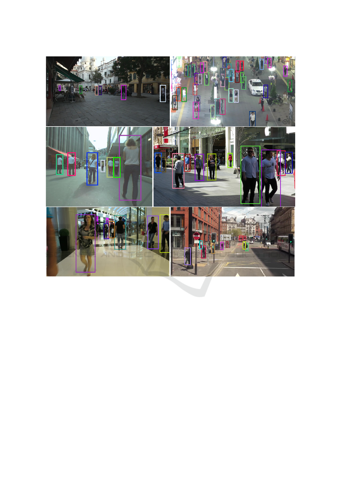
Figure 1: Sample results on several sequences of MOT16 datasets, bounding boxes represents the tracking results with

their color-coded identities. From left to right: MOT16-01, MOT16-03 (top row), MOT16-06, MOT16-08 (middle row),and

MOT16-12, MOT16-14 (bottom row).

Examples of tracking results of all MOT16 test

sequences except MOT16-07 are shown in Figure 1;

from left to right: MOT16-01, MOT16-03 (top row),

MOT16-06, MOT16-08 (middle row), and MOT16-

12, MOT16-14 (bottom row). Three frames from

MOT16-07 are shown in Figure 2. In all ﬁgures, the

bounding boxes represent the tracking results with

their color-coded identities. The MOT16-07 shown

in Figure 2 contains 54 tracks recorded by a moving

camera in a sequence of 500 frames. Tracking in this

sequence is a very challenging task, not only because

the density of pedestrians is quite high, but also

because signiﬁcant camera motion makes the person

trajectories to be both rough and discontinuous. Our

tracker reasonably performs even on this sequence

though some identity switches occur due to signiﬁ-

cant camera motion, detection failures and lack

of appearance model in our approach.

5 CONCLUSIONS

We have developed a novel multi-target visual tracker

based on the recently developed Hypothesized and

Independent Stochastic Population (HISP) ﬁlter.

We apply this ﬁlter for tracking multiple targets in

video sequences acquired under varying environ-

mental conditions and targets density. We followed

a tracking-by-detection approach using the public

detections provided in the Multiple Object Tracking

2016 (MOT16) benchmark datasets. We also allevi-

Online Multi-target Visual Tracking using a HISP Filter

435

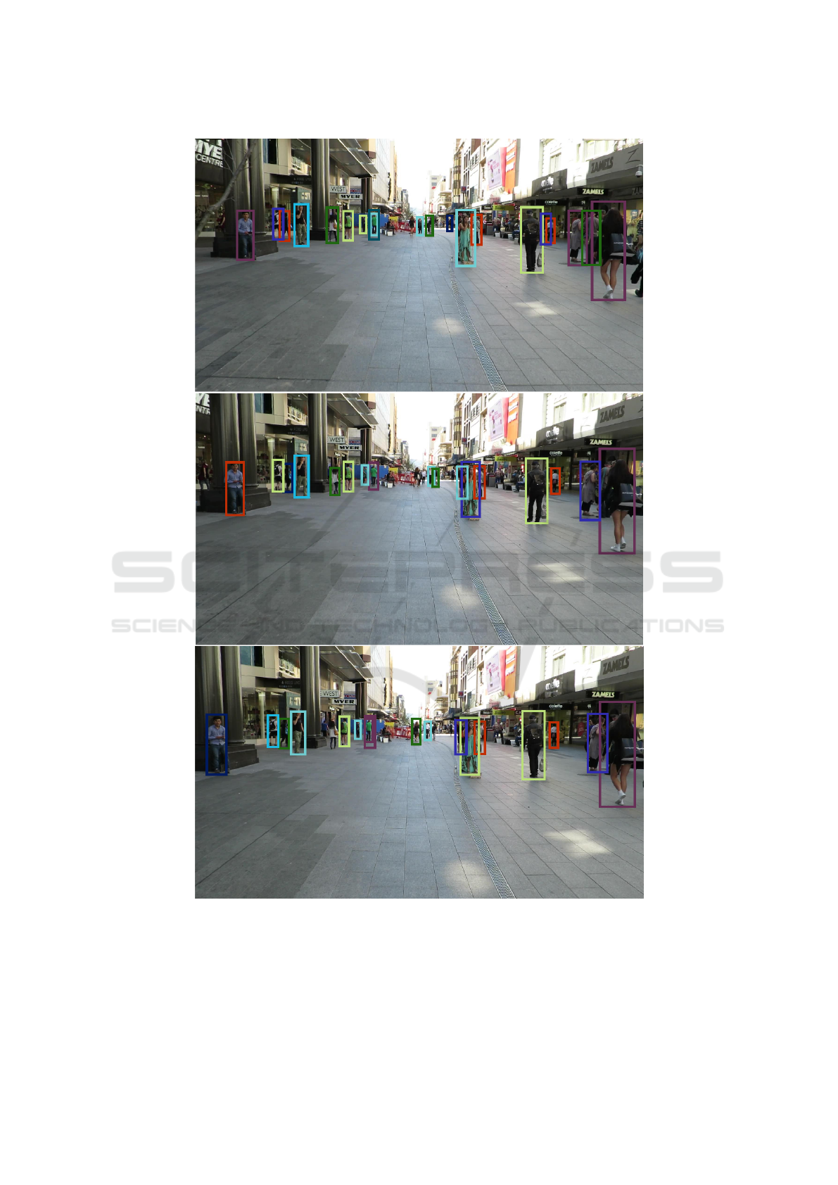
Figure 2: Sample results on the sequence MOT16-07, bounding boxes represents the tracking results with their color-coded

identities, for frames 354, 368 and 380 from top to bottom.

ate the problem of identical labels that two or

more nearby targets share through the employed

track extraction approach by using the weight of the

conﬁrmed tracks which is very crucial in the case

of video tracking. Results show that our method

outperforms state-of-the-art trackers developed using

both online and ofﬂine approaches on the MOT16

benchmark datasets in terms of tracking accuracy.

VISAPP 2018 - International Conference on Computer Vision Theory and Applications

436

Table 1: Tracking performance of representative trackers

developed using both online and ofﬂine methods. All trac-

kers are evaluated on the test dataset of the MOT16 (Milan

et al., 2016) benchmark using public detections. The ﬁrst

and second highest values are highlighted by bold and un-

derline.

Tracker Tracking Mode MOTA↑ MOTP↑ MT (%)↑ ML (%)↓ FP↓ FN↓ IDS↓ Frag↓

CEM (Milan et al., 2014) ofﬂine 33.2 75.8 7.8 54.4 6,837 114,322 642 731

DP-NMS (Pirsiavash et al., 2011) ofﬂine 32.2 76.4 5.4 62.1 1,123 121,579 972 944

SMOT (Dicle et al., 2013) ofﬂine 29.7 75.2 5.3 47.7 17,426 107,552 3,108 4,483

JPDF-m (Rezatoﬁghi et al., 2015) ofﬂine 26.2 76.3 4.1 67.5 3,689 130,549 365 638

GM-PHD-MA (Song and Jeon, 2016) online 30.5 75.4 4.6 59.7 5,169 120,970 539 731

HISP-T (ours) online 35.9 76.1 7.8 50.1 6,406 107,905 2,592 2,299

The tracker works at an average speed of 4.8 fps. In

the future work, we will use appearance features,

either hand-engineered or deep learning, to alleviate

identity switches and trajectory fragmentation.

REFERENCES

Baisa, N. L., Bhowmik, D., and Wallace, A. (2017). Long-

term correlation tracking using multi-layer hybrid fe-

atures in dense environments. In Proceedings of the

12th International Conference on Computer Vision

Theory and Applications (VISAPP), VISIGRAPP.

Baisa, N. L. and Wallace, A. (2017). Multiple Target, Multi-

ple Type Filtering in RFS Framework. ArXiv e-prints.

Baisa, N. L. and Wallace, A. (2017). Multiple target, multi-

ple type visual tracking using a Tri-GM-PHD ﬁlter. In

Proceedings of the 12th International Conference on

Computer Vision Theory and Applications (VISAPP),

VISIGRAPP.

Cham, T.-J. and Rehg, J. M. (1999). A multiple hypothesis

approach to ﬁgure tracking. In CVPR, pages 2239–

2245. IEEE Computer Society.

Delande, E., Houssineau, J., and Clark, D. (2016). Multi-

object ﬁltering with stochastic populations. arXiv,

1501.04671v2.

Delande, E., Houssineau, J., Franco, J., Frh, C., and Clark,

D. (2017). A new multi-target tracking algorithm for

a large number of orbiting objects. 27th AAS/AIAA

Space Flight Mechanics Meeting.

Dicle, C., Camps, O. I., and Sznaier, M. (2013). The way

they move: Tracking multiple targets with similar ap-

pearance. In 2013 IEEE International Conference on

Computer Vision, pages 2304–2311.

Houssineau, J. and Clark, D. (2016). Multi-target ﬁltering

with linearised complexity. arXiv, 1404.7408v2.

Houssineau, J., Clark, D. E., and Del Moral, P. (2015). A se-

quential monte carlo approximation of the HISP ﬁlter.

In Signal Processing Conference (EUSIPCO), 2015

23rd European, pages 1251–1255. IEEE.

Kasturi, R., Goldgof, D., Soundararajan, P., Manohar, V.,

Garofolo, J., Bowers, R., Boonstra, M., Korzhova, V.,

and Zhang, J. (2009). Framework for performance

evaluation of face, text, and vehicle detection and

tracking in video: Data, metrics, and protocol. IEEE

Transactions on Pattern Analysis and Machine Intel-

ligence, 31(2):319–336.

Leal-Taix, L., Canton-Ferrer, C., and Schindler, K. (2016).

Learning by tracking: Siamese CNN for robust tar-

get association. IEEE Conference on Computer Vision

and Pattern Recognition Workshops (CVPR). DeepVi-

sion: Deep Learning for Computer Vision.

Li, Y., Huang, C., and Nevatia, R. (2009). Learning to asso-

ciate: Hybridboosted multi-target tracker for crowded

scene. In In CVPR.

Mahler, R. P. (2003). Multitarget bayes ﬁltering via ﬁrst-

order multitarget moments. IEEE Trans. on Aerospace

and Electronic Systems, 39(4):1152–1178.

Online Multi-target Visual Tracking using a HISP Filter

437

Milan, A., Leal-Taix

e, L., Reid, I., Roth, S., and Schindler,

K. (2016). MOT16: A benchmark for multi-object

tracking. arXiv:1603.00831 [cs]. arXiv: 1603.00831.

Milan, A., Roth, S., and Schindler, K. (2014). Continuous

energy minimization for multitarget tracking. IEEE

Transactions on Pattern Analysis and Machine Intel-

ligence, 36(1):58–72.

Pirsiavash, H., Ramanan, D., and Fowlkes, C. C. (2011).

Globally-optimal greedy algorithms for tracking a va-

riable number of objects. In CVPR 2011, pages 1201–

1208.

Rasmussen, C. and Hager, G. D. (2001). Probabilistic data

association methods for tracking complex visual ob-

jects. IEEE Transactions on Pattern Analysis and Ma-

chine Intelligence, 23:560–576.

Rezatoﬁghi, S. H., Milan, A., Zhang, Z., Shi, Q., Dick, A.,

and Reid, I. (2015). Joint probabilistic data associa-

tion revisited. In 2015 IEEE International Conference

on Computer Vision (ICCV), pages 3047–3055.

Sanchez-Matilla, R., Poiesi, F., and Cavallaro, A. (2016).

Online multi-target tracking with strong and weak de-

tections. In Computer Vision - ECCV 2016 Workshops

- Amsterdam, The Netherlands, October 8-10 and 15-

16, 2016, Proceedings, Part II, pages 84–99.

Song, Y. and Jeon, M. (2016). Online multiple object

tracking with the hierarchically adopted GM-PHD ﬁl-

ter using motion and appearance. In IEEE/IEIE The

International Conference on Consumer Electronics

(ICCE) Asia.

Vo, B.-N. and Ma, W.-K. (2006). The Gaussian mixture

probability hypothesis density ﬁlter. Signal Proces-

sing, IEEE Transactions on, 54(11):4091–4104.

VISAPP 2018 - International Conference on Computer Vision Theory and Applications

438