Leveraging the Spatial Label Structure for Semantic Image Labeling

using Random Forests

Manuel W

ollhaf, Ronny H

ansch and Olaf Hellwich

Computer Vision & Remote Sensing, Technische Universit

at Berlin, Berlin, Germany

Keywords:

Random Forests, Semantic Segmentation, Structured Prediction, Context Information.

Abstract:

Data used to train models for semantic segmentation have the same spatial structure as the image data, are

mostly densely labeled, and thus contain contextual information such as class geometry and cooccurrence.

We aim to exploit this information for structured prediction. Multiple structured label spaces, representing

different aspects of context information, are introduced and integrated into the Random Forest framework.

The main advantage are structural subclasses which carry information about the context of a data point. The

output of the applied classiﬁcation forest is a decomposable posterior probability distribution, which allows

substituting the prior by information carried by these subclasses. The experimental evaluation shows results

superior to standard Random Forests as well as a related method of structured prediction.

1 INTRODUCTION

Contextual information plays a major role within the

human vision system (Hock et al., 1974; Biederman

et al., 1982) and enhances results in a variety of com-

puter vision tasks. However, the speciﬁc role of con-

text in image understanding and how to embed con-

textual information in corresponding methods is still

an open research question. We aim to improve se-

mantic segmentation results using semantic context

information and gain insights about how this infor-

mation contributes to the learning and inference pro-

cess. To gather these semantic contextual relations

we leverage the spatial structure of pixelwise labeled

training data.

The basis of most machine learning approaches

on semantic segmentation is a sliding window clas-

siﬁcation. These classiﬁers usually use features that

expose textural context information but do not at-

tempt to induce a meaningful structure in the out-

put space in an explicit manner. Recent work tackles

this mostly by topping the output of the classiﬁer

with a second model to capture the structural infor-

mation (Shotton et al., 2006; Mottaghi et al., 2014).

These additional processing modules are probabilis-

tic graphical models which represent the spatial rela-

tionship of classes either as a Markov Random Field

(MRF) or as the pairwise potential of a Conditional

Random Field (CRF) (He et al., 2004). Using such

a sophisticated model allows to learn the structure of

the output space in every conceivable detail, including

smoothness assumptions, class context, or geometri-

cal relations and location priors. Inference on these

models is NP-hard in general and requires algorithms

that ﬁnd approximate solutions like spatially limited

inference (Nowozin and Lampert, 2011). Our work

provides an alternative approach that integrates clas-

siﬁcation and structured prediction in a single learner.

This is accomplished by employing a Random Forest

(RF) that allows to combine both concepts in an in-

tuitive and comprehensible way. In contrast to our

work, most current work is based on deep learning in

the form of convolutional networks (ConvNets) (Long

et al., 2015; Lin et al., 2016). Their astonishing per-

formance is rooted in successive transformations of

the input data into feature spaces with increasing ab-

straction and meaningfulness. In terms of deep le-

arning, the ability to learn the parameters of a split

function adds one layer of feature transformation and

makes RFs a rather shallow learner with a depth of

two, while ConvNets usually consist of ten and more

layers. However, this large number of layers makes

huge amounts of training data necessary and requi-

res extraordinary computing capabilities, whereas our

work aims to improve segmentation results through a

more efﬁcient use of training data. Besides this, the

natural handling of multi-class problems, the proba-

bilistic output, and their almost ideal statistical pro-

perties (Hastie et al., 2009) make RFs an attractive

method for semantic segmentation.

Wöllhaf, M., Hänsch, R. and Hellwich, O.

Leveraging the Spatial Label Structure for Semantic Image Labeling using Random Forests.

DOI: 10.5220/0006546801930200

In Proceedings of the 13th International Joint Conference on Computer Vision, Imaging and Computer Graphics Theory and Applications (VISIGRAPP 2018) - Volume 5: VISAPP, pages

193-200

ISBN: 978-989-758-290-5

193

Figure 1: Application of context information on different spatial scales. From left to right: Image and ground truth, local,

small-scale, large-scale, global, and combined.

To use contextual information in a way that allows

efﬁcient learning and inference, our work uses dom-

ain speciﬁc assumptions about relevant spatial scales

and the corresponding types of context. Label infor-

mation is categorized in four spatial classes: Local,

small-scale, large-scale, and global (Fig. 1). Our

work evaluates if and how these types of informa-

tion can be predicted from local appearance to allow

their integration into a simple patch-based semantic

segmentation method. All categories are evaluated

separately and are subsequently integrated into one

model. The details of the proposed method are ex-

plained in Section 3. The ﬁrst kind of information,

called local label information, is the atomic class la-

bel that corresponds to an image patch. The second,

the small-scale information, is harnessed using a met-

hod introduced in (Kontschieder et al., 2011; Kont-

schieder et al., 2014). It uses label patches centered

at the same point as the image patch and represents

regional class geometry and regional class cooccur-

rences. This regional information does not capture

relationships between distant object parts. To incor-

porate the relations of image regions on an object le-

vel, which are referred to as large-scale information,

object shape is modeled using the implicit shape mo-

del (ISM) from (Leibe et al., 2004). The Generali-

zed Hough transform, which is part of the ISM, is

integrated into RFs in a series of publications (Gall

and Lempitsky, 2009; Gall et al., 2011; Kontschie-

der et al., 2012; Gall et al., 2012; Kontschieder et al.,

2014). Since RFs allow to combine classiﬁcation and

regression, these so called Hough Forests are often

utilized to approach combined classiﬁcation and de-

tection tasks. Our work extends this concept and

uses the detector activations of Hough Forests to re-

ﬁne the segmentation. Object detection as an inter-

mediate step to reﬁne semantic segmentation has al-

ready proven to be successful. One example is the

usage of detector outputs in (Ladick

y et al., 2010) as

additional potentials for a CRF to reﬁne a semantic

segmentation and allow differentiation between ob-

ject instances. In (Yang et al., 2012) the generative

model from (Felzenszwalb et al., 2010) is used to im-

prove segmentations with the aid of detector activati-

ons. The works in (Gu et al., 2009; Arbel

aez et al.,

2012) use region-based object detectors and combine

the region proposals to a semantic segmentation using

the generated object hypotheses. Our work integra-

tes a discriminative approach on object detection and

semantic segmentation. Already (Leibe et al., 2004)

does not only introduce the ISM, but also use the pre-

dicted object hypotheses for a ﬁgure-ground segmen-

tation. Both of these parts are adopted in our work

and extended for the use in multi-class semantic seg-

mentation. However, the closed probabilistic formu-

lation for the segmentation in (Leibe et al., 2004) is

limited to pixels that were involved in the voting pro-

cess of the Hough transfrom. We propose an alterna-

tive probabilistic method that allows to propagate evi-

dence given by object hypotheses into a convex hull

formed by the voters of a hypothesis. On a fourth spa-

tial scale, global context is introduced by learning the

statistical relation between local appearance and the

global, image wide class distribution.

As it is possible to train a Random Forest model

on multiple label spaces, the model allows multiple

simultaneous predictions each representing an aspect

of contextual information corresponding to one of the

above mentioned categories. The different predictions

are combined using the maximum a posteriori formu-

lation of the classiﬁcation problem:

y = f (x

x) = argmax

p(x

x|y

y)p(y

y). (1)

The posterior contains semantic context as the joint

probabilities of the label variables y

y = (y

,...,y

Hence, likelihood and prior of the Bayesian decom-

position of the posterior can be interpreted as appea-

rance and context as in (Tu, 2008). Random Fore-

sts allow to decompose the posterior and to adopt this

view.

Summarizing the contribution of this work:

• We incorporate the prediction of large-scale and

global context information into the Random Fo-

rest framework.

• A comparison of small-scale, large-scale, and

global context information shows similar perfor-

mance improvements for all evaluated spatial sca-

les.

• Combining predictions on different spatial scales

leads to a signiﬁcant improvement compared to

the reference method.

VISAPP 2018 - International Conference on Computer Vision Theory and Applications

194

2 RANDOM FORESTS

Random Forests (RFs) are ensembles of decision

trees that are hierarchical structures of leaf- and split-

nodes used for classiﬁcation and regression (Breiman,

2001). While the leaves contain the actual predicti-

ons, the split nodes are binary test functions f

with

parameter vector θ ∈ T , propagating a data point

x ∈ X to one of two sub-trees:

(x) =

(

1, if φ(x) ≥ τ

0, otherwise.

(2)

Here τ is a threshold value. A common choice for

φ(x) is the (absolute) difference of two pixels around

the pixel coordinates u:

φ(x) = |x

(u + b) − x

(u + a)|, (3)

which is an approximation of the gradient on the con-

necting line between a and b and thus a simple edge

detector. In this example, the additional parameter c

describes the color channel of the image x

x resulting

in θ = (a,b,c, τ). For this work φ is drawn randomly

from a set of four different functions (see supplemen-

tary material

To generate a tree, the training data S

is split

successively. Each split is chosen in a way such that

the resulting subsets S

and S

are as pure as possible

regarding the class label. This purity is measured with

an objective function such as the information gain I

using the Shannon entropy H:

= H(S ) −

∑

i∈{0,1}

|S|

· H(S

). (4)

For an optimal split at node k, the second term of

the information gain, the sum of the weighted en-

tropies of the resulting subsets, must be minimized.

While an entropy-based objective function for regres-

sion is possible, regression forests usually choose a

split that minimizes the variance within the resulting

subsets for simplicity and to lower the computational

costs (Criminisi et al., 2012; Gall et al., 2012). The

objective function for the regression label spaces is

deﬁned as

= argmin

θ∈T

∑

i∈{0,1}

∑

y∈Y

∑

d∈S

(d − d)

, (5)

where Y is the set of labels and d the mean of the tar-

get variable for regression (e.g. offset vectors) in S

The normalization with the sample size usually found

in the variance equation is missing since the sub-

sets are weighted with their size to avoid unbalanced

Supplementary material can be found under: http://

rhaensch.de/structuredRF.html

splits. As it is not necessary to reduce the variance be-

tween data points belonging to different classes, this

formula is extended to only consider intraclass vari-

ance for forests in which classiﬁcation and regression

are combined as in (Gall et al., 2011). The use of

variance minimization implies a unimodal data dis-

tribution. This assumption is often invalid. As in

most works this objective is chosen in the absence of

a computational tractable alternative for multimodal

distributions.

A leaf node is created if there are less than a cer-

tain number of samples in the subset left, the maxi-

mum tree depth is reached, or the subset is pure. Each

leaf stores a representation of the remaining data sam-

ples. Forests used for semantic segmentation usually

store the class frequency of the subset. As an approx-

imation of the posterior, this distribution includes the

prior distribution of the training data according to the

Bayes’ theorem. To allow to train the model with un-

balanced data the distribution gets re-balanced with

the reciprocal prior distribution

|S|

/|S

All trees are trained independently and their out-

put is averaged for inference. The single trees are

randomized by choosing the optimal split only from

a relatively small subset of created split candidates by

randomly sampling split parameters θ. This proce-

dure leads to a very efﬁcient training on high dimen-

sional data.

3 METHOD

This work aims to exploit topological information

from the label space with the aid of Random Forests

(RFs). Therefore, information on local, small-scale,

large-scale, and global level is incorporated into dif-

ferent structured label spaces, used as split criteria for

the tree nodes, stored in the leaf nodes, and combi-

ned into a consistent pixelwise class prediction. A

detailed description of implementation decisions and

parameter choices can be found in the supplementary

material

Structured Labels in RFs. The ﬁrst step of the pro-

posed approach is to deﬁne a representation of the

context information contained in the structure of the

pixelwise labeled data. Local information is the ato-

mic label y = (u, y

y) corresponding to the center of a

data point (image patch) x = (u,r,x

x). Here u is the pa-

tch center, r the patch shape, x

x the image, and y

y the la-

bel image. This label representation does not contain

any topological information. Small-scale information

denotes a small region r

in y

y around u corresponding

Leveraging the Spatial Label Structure for Semantic Image Labeling using Random Forests

195

void sky grass tree cow

Class

Occurrence

Figure 2: Training data and structured labels. (left) Image with emphasized image patch. (middle) Label image with empha-

sized small-scale and large-scale information. (right) Global context label.

to a data point x (Fig. 2 middle). Note that the re-

gion r

has not necessarily the same size as region r

the image patch in x

x, but is centered at the same posi-

tion u. This label type is introduced in (Kontschieder

et al., 2011) and (Kontschieder et al., 2014). As labels

on the large-scale level, the well known Hough featu-

res are deployed (Leibe et al., 2004) (Fig. 2 middle).

Here, a Hough feature is an offset vector d describing

the displacement between u and the object center and

thus depicts the geometrical structure of the label in-

formation on an object level. Global, image level in-

formation is incorporated by assigning the same label

to every image patch, namely the image wide class

distribution (Fig. 2 right).

Training Objective. RFs can be utilized for clas-

siﬁcation and regression. A single RF can be trai-

ned using multiple different label spaces from both

problem classes by randomly selecting a label space

in each split-node. The split-nodes split the data set

using an objective function appropriate to the selected

label space. The concept from Eq. 4 can be directly

applied for the local labels. The small-scale label is

handled by randomly choosing two atomic labels for

each split node and separate the data by maximizing

the joint information gain. As suggested in (Kont-

schieder et al., 2011), choosing the center pixel as one

of the compared pixels ensures the separation of the

data by local information. Large-scale and global la-

bels are handled as a regression problem. The histo-

grams for the global labels are therefore interpreted as

data points with dimensions of the number of classes.

Leaf Nodes. To leverage the topological informa-

tion in the label space a representation of the structu-

red labels which are used to split the data sets must

also be preserved. Of the small-scale label patches

which set up a leaf node Kontschieder et al. use only

the one that represents the set of labels best. The

best representation is determined with an approxima-

tion of the joint probability assuming independence

between pixels. This approach allows to keep the

memory consumption of the tree acceptable despite

the high dimensional label. This work adopts this

method. The large-scale information is preserved

in the leaf nodes as a non-parametric spatial density

distribution p(v|x). A sparse representation of the

occurring coordinates (non-zero densities) describes

the distribution in a simple and detailed way, even if

the distribution is multimodal. The global label is an

additional histogram which is the average of the his-

tograms of class densities. Output distributions of dif-

ferent trees are combined by averaging. The predicti-

ons of the small-scale labels are uniﬁed over multiple

trees by maximization of the joint probability.

Prediction from Structured Labels. After a RF in-

stance is trained on one or more label spaces, the pre-

dictions ˆy about class distributions and label structure

must be fused into a meaningful result. This work

evaluates several prediction processes based on diffe-

rent label types. The normalized local class distribu-

tion, inferred from the prediction based on the local

label, is referred to with p

as it is proportional to the

likelihood term of the Bayes’ formula. Small-, large-

scale, and global information are used to generate dis-

tributions which are supposed to enforce a regional

resp. global compliance to the predicted structural

properties of the image patch. The large-scale and

global distributions are combined with p

in the hope

of achieving a posterior distribution which expresses

a per pixel class prediction consistent with large-scale

and global structure of the image. As the small-scale

label already contains local information, there is no

need for a combination with a distribution generated

from local information.

The small-scale information is transformed into a

position dependent distribution p(y,u) by fusing pre-

dictions from neighboring pixels to encourage a regi-

onal consensus. The neighborhood is deﬁned as the

set of pixels in the region r

which is the label patch

centered at u. The distribution at u generated from the

small-scale labels is a voting of all labels correspon-

ding to pixels in r

p(y|u) =

∑

v∈r

[ ˆy(v,u) = y] (6)

This procedure is referred to as simple fusion process

in (Kontschieder et al., 2011).

VISAPP 2018 - International Conference on Computer Vision Theory and Applications

196

The attempt to reach a consistent prediction on

large-scale level is based on the idea that patches,

which belong to the same object, should make a mos-

tly coinciding prediction about the objects centers po-

sition. Therefore, an estimate about the position of

the object center for all patches of an image is col-

lected. The object hypotheses the most patches agree

on are used to encourage a classiﬁcation of the single

patches which is conform to these hypotheses. Note,

that the actual position of the hypothesis is not impor-

tant as it is not used for object detection or objectwise

segmentation. For the generation of the large-scale

prior two different methods are evaluated and com-

pared. First, the forest is trained on the atomic and

the Hough labels and thus associates a class distribu-

tion p(y|x) and a spatial distribution p(v|x) with each

image patch x. The joint distribution p(y,v|x) of both

describes the hypothesis of the position v of an object

center and corresponding object class y. These dis-

tributions are used for a voting in a Hough space for

which all hypotheses of all image patches are summed

up:

H (y,v) =

∑

x∈x

p(y,v|x) =

∑

x∈x

p(y|x)p(v|x) (7)

The n most prominent maxima h

1...n

in the voting

space are selected using the maximum of the class

distribution for each pixel position. Given this list of

hypotheses all voters V

1...n

that voted for one of the

peaks are identiﬁed (see supplementary material

The ﬁrst of the two evaluated methods generates

a convex hull from these voters for each hypothesis

and assigns the average local class distribution of the

voters to each pixel within the hull:

(y|h

,u) =

∑

v∈V

(v). (8)

Pixels outside the convex hull are treated as having

an uniformly distributed class prior. A weighted and

re-normalized sum of these distributions results in the

ﬁnal prior distribution:

(y|u) =

∑

l=1

H (h

)

∑

l=1

(y|h

,u)H (h

) (9)

The second method is supposed to integrate small-

scale and large-scale information and therefore adopts

the probabilistic formulation from (Leibe et al., 2004)

to combine Generalized Hough Transformation and

semantic segmentation. The implicit shape model

(ISM) described in (Leibe et al., 2004) uses a code-

book inferred from the training data for the Hough

voting. Image patches trigger a number of codebook

entries which pass votes into the voting space. Ad-

ditionally, a set of segmentation masks is stored with

the codebook entries. The segmentation masks im-

plement the small-scale inﬂuence, i.e. p(y|h

,u,x)

reﬂects if u lies within the mask associated with x.

We adopt this part through a small-scale prediction,

using a model that is additionally trained on a bina-

rized small-scale label. As binary matrix it marks all

pixels of y

y in the region r that have the same class la-

bel as position u and describes the spatial distribution

of the class in the region.

For this method the prior is formulated as distri-

bution conditioned on an object hypothesis and mar-

ginalized over image patches x:

(y|h

,u) =

∑

x∈x

p(y|h

,u,x)p(x|h

,u) (10)

The ﬁrst term describes the small-scale inﬂuence of

the image patch x on the class distribution at pixel u.

It is weighted with the contribution of the patch to

the object hypothesis h

. As only patches contai-

ning u have small-scale inﬂuence p(y|u, x) > 0 and

only patches that voted for h

have non-zero weight

p(x|h

) > 0, the sum reduces to the intersection of

these subsets.

(y|h

,u) =

∑

x∈r

p(y|h

,x)p(x|h

) (11)

∑

x∈r

p(y|h

,x)

p(h

|x)p(x)

p(h

)

(12)

Assuming a uniform distribution for the priors p(x)

and p(h) one can substitute the term p(x|h

) with

p(h

|x) = p(y

|x) from Eq. 7. Finally the priors ge-

nerated for each hypothesis are combined as in Eq. 9.

The global probability density describing the

image wide class occurrence is independent of the

image coordinates u. It is deﬁned as the mean of the

global labels estimated for the patches of an image x

This prior encourages an image wide consensus about

which classes are likely to appear in the scene.

(y) =

∑

v∈x

ˆy(v) (13)

4 EXPERIMENTS

The forests are trained and evaluated on

MSRCv2 (Shotton et al., 2006) data set, which

contains 276 training, 59 validation, 256 test images

and 21 object classes. Images are fed into the RF

using LAB color space and with nine additional

HOG-like feature channels (see supplementary

material

). Due to the grid sampling strategy (5×5),

the resulting set of data points is unbalanced. Three

metrics are listed for each experiment to evaluate the

Leveraging the Spatial Label Structure for Semantic Image Labeling using Random Forests

197

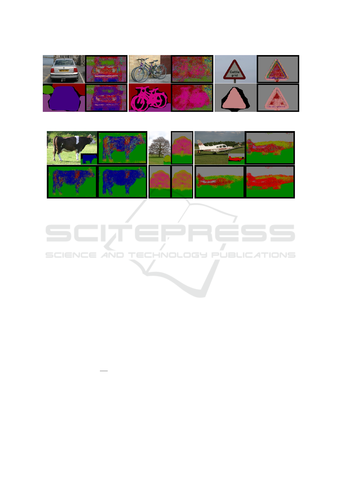
Figure 3: Results for the (convex-hull) large-scale prior. (top-left) Original image (top-right) Likelihood. (bottom-left) Ground

truth. (bottom-right) Posterior.

Figure 4: Results for global prior. (top-left) Original image. (top-right) Likelihood. (bottom-left) Global consensus prior.

(bottom-right) Posterior.

results besides a qualitative analysis. These are the

global recall (GR), the average recall (AR), and the

average intersection over union or average Jaccard

index (AJ) (Everingham et al., 2010). The baseline

for the experiments is a standard Random Forest

model without modiﬁcations. The forest parameters

are: Number of trees T = 10, maximum tree depth

D = 99, and minimum number of samples S

min

= 5.

All data points from the training set are used for the

training of all trees (i.e. no bagging). We ﬁxed the

feature patch size for all experiments to 21 × 21 and

the small-scale label patch size to 11 × 11.

As a baseline, additional to the classiﬁcation re-

sults based on the local label, the results for three

posterior distributions are given: Consensus (small-

scale), consensus (global), and consensus (both).

These three posterior distributions are generated with

three uninformed prior distributions. They enforce a

consensus in the classiﬁcation result but incorporate

no knowledge inferred from the training data. They

are deﬁned as an average of the local class distributi-

ons p

(y|u) =

∑

v∈r

(v). (14)

For the consensus (small-scale) posterior, r

is a re-

gion around the pixel coordinates u with the same

size as the small-scale label patch to enforce a consen-

sus of the class distributions on this spatial scale. A

global consensus is encouraged with the mean of all

patchwise predictions throughout the image r

= x

The combination of the consensus (small-scale) and

consensus (global) priors is denoted with consensus

(both). These posterior distributions are intended to

allow a more meaningful interpretation than a com-

parison to an arbitrary CRF model.

Results. The results for the integration of small-

scale information are very similar to those published

in (Kontschieder et al., 2014). They are slightly better

than the results achieved with the uninformed small-

scale consensus prior (Table 1). Note that this com-

parison concerns only the simple fusion process sug-

gested by Kontschieder et al..

Large-scale information is exploited using two

different approaches: Convex hull & ISM. The ﬁrst

method surpasses the results achieved with the small-

scale label (for the AR and AJ score), the small-scale,

and the global baseline-priors. It even outperforms

the combination of both baseline-priors wrt. AR. Fi-

gure 3 emphasizes how a weak signal in the local-

appearance-based classiﬁcation can lead to a robust

and correct classiﬁcation of a region. This conﬁrms

previous ﬁndings that object detection can improve

semantic segmentations and shows that the propo-

sed method is effective. The second method leads

to an improvement too, but cannot compete with the

convex-hull-based method. One reason for the com-

parably low performance is the property of the appro-

ach to propagate the knowledge about object hypot-

VISAPP 2018 - International Conference on Computer Vision Theory and Applications

198

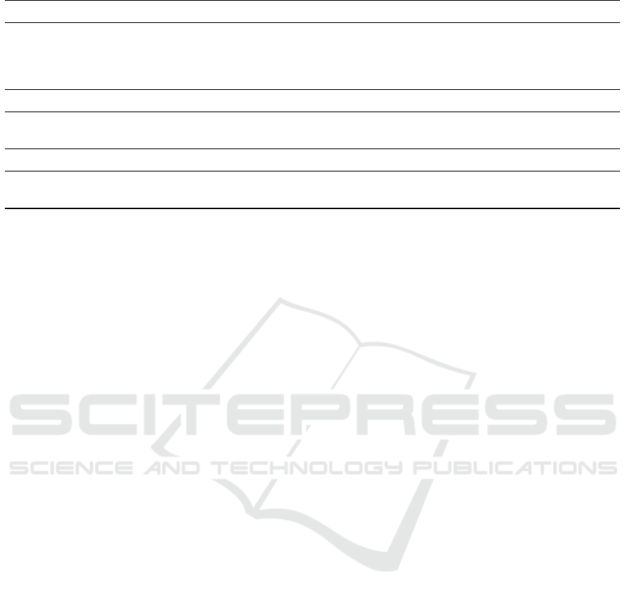
Table 1: Results for baseline, different spatial scales and a combination of those.

GR AR AJ

baseline

likelihood 57.06 39.73 27.86

consensus (small-scale) 61.67 44.20 31.87

consensus (global) 63.23 44.27 33.16

consensus (both) 65.09 46.25 34.88

small-scale 63.56 47.17 33.94

large-scale

convex hull 61.50 49.61 34.67

ISM 58.27 43.84 30.22

global 63.83 49.69 35.71

combinations

local & convex hull & global 65.81 54.09 39.37

small & convex hull & global 66.94 57.86 40.77

heses in a local region around the voters.

The prior formulated using the patch-based pre-

dictions about the global class distribution outper-

forms the uninformed prior. Furthermore, it outper-

forms the results achieved by incorporating small-

scale and large-scale information. This shows that it

is possible to infer global image properties from lo-

cal appearance and to use this knowledge to improve

semantic segmentations. The qualitative analysis in

Figure 4 shows signiﬁcantly better results for the in-

formed global prior compared to the uninformed glo-

bal consensus prior.

The convex-hull-based large-scale and the global

prior are combined and evaluated two times: On ba-

sis of local information and using small-scale infor-

mation as a basis for the large-scale prior. The com-

bination of large-scale and global information shows

to be hardly redundant. It leads to remarkable results

with a relative improvement of 40% for AJ compa-

red to the standard model. Even the slight decrease

of the GR score, comparing the baseline priors and

large-scale prior, is compensated by the combination

of both information levels. An additional combina-

tion with small-scale information improves the results

further, but at the cost of memory footprint computa-

tional load.

5 CONCLUSION

We leverage the spatial label structure of densely la-

beled image data to support the learning and inference

process of RFs for semantic segmentation. Different

structured labels are introduced that exploit contex-

tual information encoded at different spatial scales:

Small-scale, large-scale, and global. While the small-

scale level is based on (Kontschieder et al., 2011;

Kontschieder et al., 2014), the large-scale information

is introduced by a Hough-voting-based object detec-

tor. This leads to enhanced segmentations compared

to the baseline and performes on par with the refe-

rence method (Kontschieder et al., 2014). Similar

results are achieved through incorporation of global

context information. A combination of both introdu-

ced methods and of all three spatial scales improves

the results considerably, with a relative improvement

of 40% for the average Jaccard index compared to the

standard Random Forest model and 20% compared to

the reference method. Our work shows how to har-

ness the structure of the label space, to integrate con-

text information on different scales and demonstrates

that the potential of RFs is not yet exhausted.

Future Work. This work leaves multiple ways to

counteract the shortcomings of the ISM-based met-

hod to integrate large-scale information to further eva-

luation. One way is to increase the size of the used

small-scale label. Another is to use a less restrictive

voter identiﬁcation process. Further development to

reﬁne this approach would be worthwhile because it

has the potential to overcome the weak-point of the

convex-hull-based method: Using the convex hull as

basis for the top-down distribution of the detector

activations leads to an overestimation of the object

size, i.e. false positive classiﬁcation of background

classes as ”thing” classes. A further way to improve

the results would be to use a non-convex hull, i.e. a

polygon. Additionally both methods could proﬁt from

a substitution of the standard Hough voting, which

needs the ﬁne tuning of many parameters, with the

closed probabilistic formulation from (Barinova et al.,

2012).

REFERENCES

Arbel

aez, P., Hariharan, B., Gu, C., Gupta, S., Bourdev, L.,

and Malik, J. (2012). Semantic segmentation using re-

Leveraging the Spatial Label Structure for Semantic Image Labeling using Random Forests

199

gions and parts. In Computer Vision and Pattern Re-

cognition (CVPR), 2012 IEEE Conference on, pages

3378–3385.

Barinova, O., Lempitsky, V., and Kholi, P. (2012). On de-

tection of multiple object instances using hough trans-

forms. IEEE Transactions on Pattern Analysis and

Machine Intelligence, 34(9):1773–1784.

Biederman, I., Mezzanotte, R. J., and Rabinowitz, J. C.

(1982). Scene perception: Detecting and judging ob-

jects undergoing relational violations. Cognitive Psy-

chology, 14(2):143 – 177.

Breiman, L. (2001). Random forests. Machine Learning,

45(1):5–32.

Criminisi, A., Shotton, J., and Konukoglu, E. (2012). De-

cision forests: A uniﬁed framework for classiﬁcation,

regression, density estimation, manifold learning and

semi-supervised learning. Found. Trends. Comput.

Graph. Vis., 7(2):81–227.

Everingham, M., Van Gool, L., Williams, C. K. I., Winn,

J., and Zisserman, A. (2010). The pascal visual ob-

ject classes (voc) challenge. International Journal of

Computer Vision, 88(2):303–338.

Felzenszwalb, P. F., Girshick, R. B., McAllester, D., and

Ramanan, D. (2010). Object Detection with Discrimi-

natively Trained Part-Based Models. IEEE Transacti-

ons on Pattern Analysis and Machine Intelligence,

32(9):1627–1645.

Gall, J. and Lempitsky, V. (2009). Class-speciﬁc hough fo-

rests for object detection. In Computer Vision and

Pattern Recognition, 2009. CVPR 2009. IEEE Con-

ference on, pages 1022–1029.

Gall, J., Razavi, N., and Gool, L. V. (2012). An Introduction

to Random Forests for Multi-class Object Detection.

In Outdoor and Large-Scale Real-World Scene Ana-

lysis, number 7474 in Lecture Notes in Computer

Science, pages 243–263. Springer Berlin Heidelberg.

Gall, J., Yao, A., Razavi, N., Van Gool, L., and Lem-

pitsky, V. (2011). Hough forests for object detection,

tracking, and action recognition. Pattern Analy-

sis and Machine Intelligence, IEEE Transactions on,

33(11):2188–2202.

Gu, C., Lim, J. J., Arbelaez, P., and Malik, J. (2009). Recog-

nition using regions. In Computer Vision and Pattern

Recognition, 2009. CVPR 2009. IEEE Conference on,

pages 1030–1037.

Hastie, T., Tibshirani, R., and Friedman, J. (2009). The

Elements of Statistical Learning. Springer Series in

Statistics. Springer New York, New York, NY.

He, X., Zemel, R. S., and Carreira-Perpinan, M. A. (2004).

Multiscale conditional random ﬁelds for image labe-

ling. In Proceedings of the 2004 IEEE Computer

Society Conference on Computer Vision and Pattern

Recognition, 2004. CVPR 2004, volume 2, pages II–

695–II–702 Vol.2.

Hock, H. S., Gordon, G. P., and Whitehurst, R. (1974). Con-

textual relations: The inﬂuence of familiarity, physi-

cal plausibility, and belongingness. Perception & Psy-

chophysics, 16(1):4–8.

Kontschieder, P., Bul, S. R., Pelillo, M., and Bischof, H.

(2014). Structured labels in random forests for seman-

tic labelling and object detection. IEEE Transacti-

ons on Pattern Analysis and Machine Intelligence,

36(10):2104–2116.

Kontschieder, P., Bul

o, S. R., Criminisi, A., Kohli, P., Pe-

lillo, M., and Bischof, H. (2012). Context-sensitive

decision forests for object detection. In Pereira, F.,

Burges, C. J. C., Bottou, L., and Weinberger, K. Q.,

editors, Advances in Neural Information Processing

Systems 25, pages 431–439. Curran Associates, Inc.

Kontschieder, P., Rota Bul, S., Bischof, H., and Pelillo, M.

(2011). Structured class-labels in random forests for

semantic image labelling. In Computer Vision (ICCV),

2011 IEEE International Conference on, pages 2190–

2197. IEEE.

Ladick

y, L., Sturgess, P., Alahari, K., Russell, C., and Torr,

P. H. S. (2010). What, Where and How Many? Com-

bining Object Detectors and CRFs. In Computer Vi-

sion ECCV 2010, number 6314 in Lecture Notes in

Computer Science, pages 424–437. Springer Berlin

Heidelberg. DOI: 10.1007/978-3-642-15561-1

31.

Leibe, B., Leonardis, A., and Schiele, B. (2004). Combined

object categorization and segmentation with an impli-

cit shape model. In Workshop on statistical learning

in computer vision, ECCV, volume 2, page 7.

Lin, G., Shen, C., van den Hengel, A., and Reid, I. (2016).

Efﬁcient piecewise training of deep structured models

for semantic segmentation. In The IEEE Conference

on Computer Vision and Pattern Recognition (CVPR).

Long, J., Shelhamer, E., and Darrell, T. (2015). Fully con-

volutional networks for semantic segmentation. In

The IEEE Conference on Computer Vision and Pat-

tern Recognition (CVPR).

Mottaghi, R., Chen, X., Liu, X., Cho, N.-G., Lee, S.-W.,

Fidler, S., Urtasun, R., and Yuille, A. (2014). The

Role of Context for Object Detection and Semantic

Segmentation in the Wild. In Proceedings of the IEEE

Conference on Computer Vision and Pattern Recogni-

tion, 2014. CVPR 2014, pages 891–898.

Nowozin, S. and Lampert, C. H. (2011). Structured Le-

arning and Prediction in Computer Vision. Found.

Trends. Comput. Graph. Vis., 6(34):185–365.

Shotton, J., Winn, J., Rother, C., and Criminisi, A.

(2006). TextonBoost: Joint Appearance, Shape and

Context Modeling for Multi-class Object Recogni-

tion and Segmentation. In Leonardis, A., Bischof,

H., and Pinz, A., editors, Computer Vision ECCV

2006, number 3951 in Lecture Notes in Compu-

ter Science, pages 1–15. Springer Berlin Heidelberg.

DOI: 10.1007/11744023 1.

Tu, Z. (2008). Auto-context and its application to high-level

vision tasks. In IEEE Conference on Computer Vision

and Pattern Recognition, 2008. CVPR 2008, pages 1–

Yang, Y., Hallman, S., Ramanan, D., and Fowlkes, C. C.

(2012). Layered Object Models for Image Segmen-

tation. IEEE Transactions on Pattern Analysis and

Machine Intelligence, 34(9):1731–1743.

VISAPP 2018 - International Conference on Computer Vision Theory and Applications

200