Stability Analysis in Three Dimensions for the Incompressible
Navier-Stokes Equation
Tulus
1
, A. S. Adila
1
, T. J. Marpaung
1
, M. R. Syahputra
1
and Suriati
2
1
Department of Mathematics, Universitas Sumatera Utara, Padang Bulan 20155, Medan, Indonesia
2
Department of Informatics, Universitas Harapan Medan, H.M. Joni street 20126, Medan, Indonesia
Keywords: Navier-Stokes Equation
Abstract: This research discusses about stability on three dimensional incompressible Navier-Stokes equations in steady
state
0,
and with Navier boundary condition. The analysis is performed in a region geometrically of the
form box hollow. The result shows the shape of stability (or instability) depends on energy, and strengthen
the slip length and viscosity. With the presence of critical viscosity, it can also be shown the stability in three-
dimensional domain hold by using of normed spaces.
1 INTRODUCTION
In mathematically, the Navier-Stokes equations in
three dimensions are formed by viscosity. So, the
equations from is described by the following
system
.,
.0
where is the time, is the point of Ω; is the
density, is the velocity, is the corresponding
pressure and the positive constant is the velocity
coefficient. So,
.
The basic of stability analysis depends on which
is function ,. In the case, the autonomous
system means that the systems are not depend on the
time . Therefore,
,0,
0
The stability is defined by two Lyapunov Stability
and Asymptotic Stability (Jiang F and Jiang S, 2014).
The concept of Lyapunov stability is
is said to
be stable if given 0, there exist a
0
such that, for any other solution,
satisfying
|
|
, then
|
|
for
,
∈. The Asymptotic Stability is defined by if
there exist a constant 0 such that, if
|
|
, the lim
→
|
|
0.
There are so many researches about stability
analysis in Navier-Stokes equations, the nonlinear
instability in inhomogeneous incompressible flow
and stability and instability of gravity (Tulus, 2012).
On 2012, Tulus was obtained the stability of Taken-
Bogdanov equations with numerical solution. Based
on the research has not found any research about
stability analysis on the three dimensional for
incompressible flow. Thus, this study is about the
analysis of linear stability in the three dimensions of
the compressed Navier-Stokes equation. In this
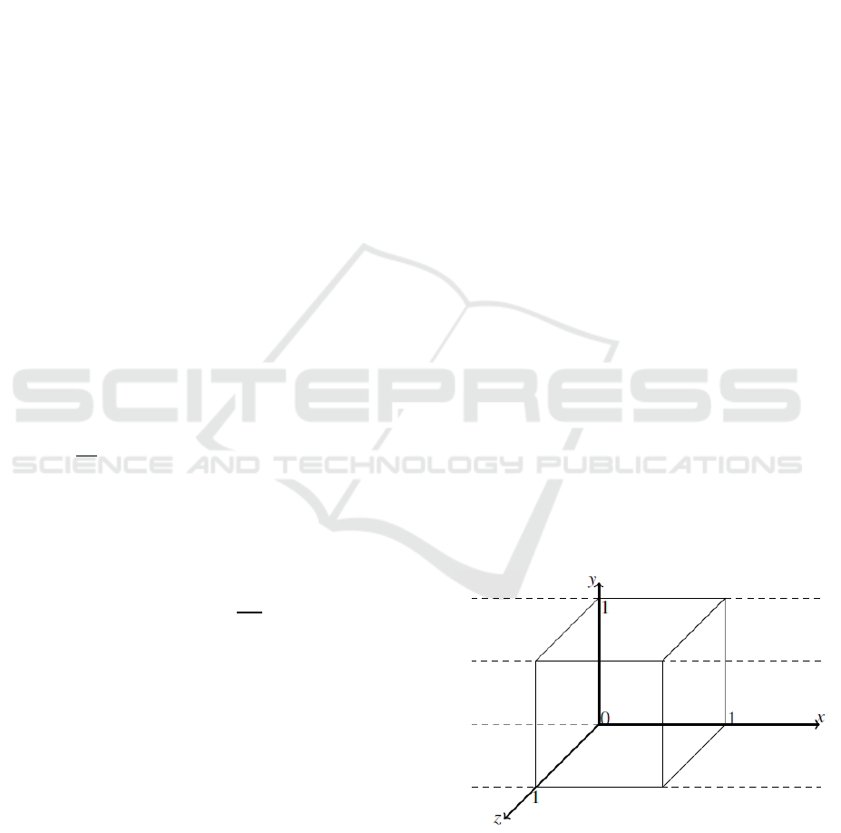
research, three-dimensional model that will be
discussed is as follows.
Figure 1:
0,1
0,1
.
Tulus, ., Aldila, A., Marpaung, T., Syahputra, M. and Suriati, .
Stability Analysis in Three Dimensions for the Incompressible Navier-Stokes Equation.
DOI: 10.5220/0010085009870990
In Proceedings of the International Conference of Science, Technology, Engineering, Environmental and Ramification Researches (ICOSTEERR 2018) - Research in Industry 4.0, pages
987-990
ISBN: 978-989-758-449-7
Copyright
c
2020 by SCITEPRESS – Science and Technology Publications, Lda. All rights reserved
987

2 METHOD
The method used in this research is
1. Define 3 dimensional incompressible
Navier- Stokes equations (Tulus et al.,
2017).
2. Define the theorems of stability and
instability (linear or nonlinear).
3. Analysis of the Navier-Stokes equation on
incompressible flow with linear stability
analysis (Tulus et al., 2018).
3 DISCUSSION
3.1 3-Dimensional Incompressible
Navier-Stokes
Given the Navier-Stokes equations for
incompressible flow
.
Δ0,
0
(1)
Where is identified as the pressure and v is the
vector field of velocity (Marpaung et al., 2018).
In this research, the Navier boundary condition is
defined on domain Ω
0,1
0,1
, then
.
Δ0;
0,1
,0,
0;0
0,1
0,1
,0
(2)
3.2 Linearization the Equation
On this research, for analysis the stability we use the
steady state on
0;
(Tulus et al., 2006).
Let is the strong solution for linearization the
equation with steady state
0,
, is the slip length,
the kinetic energy system Ε
‖
‖
. So,
based on the law of energy is
Ε
Ε
0
|
|
|
|
With 0. There are the following steps for
linearization the equation (2).
,
,
Then,
,
satisfies the following perturbed
equations:
.0
0
(3)
Therefore, the Navier boundary condition:
.0
0
(3)
Let we use the perturbation formulated as below
,0,
,1,
,,0
,,1
0,∈
(4)
,1,
,1,
,∈
(5)
,0,
,0,
,∈
(6)
,,1
,,1
,∈
(7)
,,0
,,0
,∈
(8)
Then, linearization equation (3) with steady state
,
, we obtained:
Δ0
0
(9)
3.3 Stability Analysis
For facilitate the analysis process, we will introduce
some notations,
Ω≔
0,1
0,1
,
≔
Ω
,≔,
≔
,
Ω
,
≔
∈
|div0,
0at0,10,1
Where
0,10,1 and
0,10,1 can be
written by
and
.
We will define the steady state on the equations. From
the equations (4)-(8), we obtained
,,;
,,
,
,,;
,,
(10)
For 0, substituted and w on the equation,
́0,onΩ,
di
v
0, onΩ,
(11)
We can write the and ́ in the terminology,
,,:0,10,1→ for all , we obtained:
,,
,
,,
,
́
,,
.
(12)
Elimination for the second equations (4) then
substitution the fourth order from the ODE system for
, then:
ICOSTEERR 2018 - International Conference of Science, Technology, Engineering, Environmental and Ramification Researches
988

2
,
∈0,10,1
(13)
in
f
∩
,
(14)
In this case
2
′′
2
′
2
′
1,
2
′
0,
2
′
,1
2
′
,0
and
1
2
(15)
well defined on the space
∩
For the positive ,
, then
2
′′
2
′
1,
2
′
0,
2
′
,1
2
′
,0
is negative for the viscosity . Therefore is
negative on . So, the critical viscosity is defined by
sup
∩
,
′
1,
′
0,
′′
′
,1
′
,0
′′
(16)
3.4 The Critical Viscosity
From the equation (16) we obtained the shape of the
critical viscosity,
sup
(17)
where
2
′
1,
2
′
0,
2
,
2
,
(18)
∩
|
1
2
0
1
.
Then, for every ∈
∩
,
‖
′
‖
2
‖
‖
2
,
(19)
with applied the Poincare inequality and ∈
, we
obtained the proof.
So that, for every ∈,
|
|
1
2
|
2
|
1
2
0
for every positive constant
;
, dan
depends
on
dan
. This statement proof sup
∈
is
exist and bounded. For
∶sup
∈
, we can
distinguish become two propositions
Propositions. For
∞,∞. If max
,
,
,
0 then
0
Proof. Let
,
,
and
are non-positive. Then
we have
∈,
2
1,
2
0,
2
′
,1
2
′
,0
0.
(20)
We have known the explicit from the critical
viscosity
0,
0,
0,
0,and
0
6
≔0
6
others
For
Ψ
0, ∈0,
1
4
;
exp
1
1
2
,
1
16
,∈
1
4
,
3
4
;
0, ∈
3
4
,1;
(21)
on , moreover Ψ∈
0,1,
and Ψ
1,
Ψ
0,
01, which implies
Ψ
0
implies that
0.
4 CONCLUSIONS
On this research the linear stability analysis is
obtained from the instability depends on the strength
viscosity and slip length. There are three theorems,
Stability Analysis in Three Dimensions for the Incompressible Navier-Stokes Equation
989

which are linear instability theorem, nonlinear
instability theorem, and linear stability asymptotic.
Moreover, there are the critical viscosity which
distinguish the linear stability and nonlinear
instability.
ACKNOWLEDGEMENTS
We gratefully acknowledge to all staff at Department
of Mathematics Universitas Sumatera Utara and those
who helped us to finished this research.
REFERENCES
Fei, J., Song, J., 2014. On instability and stability of three-
dimensional gravity driven viscous flows in a bounded
domain. Jornal of Advances in Mathematics. Elsevier.
Marpaung, TJ., Tulus, Suwilo, S., 2018. Cooling
optimization in tubular reactor of palm oil waste
processing. Bulletin of Mathematics. Talenta USU.
Tulus, Ariffin, AK., Sharir, A., Mohamad, N., 2006. Finite
element analysis for heat transfer in the insulator on
piston pin of a linear generator engine. 2nd IMT-GT
Regional Conference Of Mathematics, Statistics And
Applications. University Sains Malaysia.
Tulus, 2012. Numerical study on the stability of takens-
bogdanov systems. Bulletin of Mathematics. Talenta
USU.
Tulus, Suriati, Situmorang, M., Zain, DM., 2017.
Computational Analysis of Sedimentation Process in
the Water Treatment Plant. 1st International
Conference on Applied & Industrial Mathematics and
Statistics. IOP Conference Series: Materials Science
and Engineering.
Tulus, Suriati, Marpaung, TJ., 2018 Sedimentation
optimitation on river dam flow by using comsol
multiphysics. 4th International Conference on
Operational Research. IOP Conference Series:
Materials Science and Engineering.
ICOSTEERR 2018 - International Conference of Science, Technology, Engineering, Environmental and Ramification Researches
990
