A Systematic Review of Analytical Management Techniques in
Business Process Modelling for SMEs Beyond What-if-Analysis and
Towards a Framework for Integrating Them with BPM
Dimitrios A. Karras
1
and Rallis C. Papademetriou
2
1
Automation Department, Sterea Hellas Institute of Technology, P.C. 34400 Psachna, Evoia, Greece
2
Faculty Technology, University of Portsmouth, Anglesea Road, Portsmouth, PO1 3DJ, U.K.
Keywords: Business Process Modelling, Modelling Requirements, Analytical Management Techniques, Game-Theory
Modelling, Markov-Chain Modelling, Probabilistic Modelling, Cognitive Maps Modelling.
Abstract: Unquestionably, Business Process Modelling (BPM) is an increasingly popular research area for both
organisations and enterprises due to its effectiveness in enabling better planning of resources, business
reengineering and optimized business performance. The understanding of Business Process modelling is an
essential approach for an Organization or Enterprise to achieve set objectives and improve its operations.
Recent development has shown the importance of representing processes to carry out continuous
improvement. The modelling and simulation of Business Processes has been able to show Business Analysts,
and Managers where bottleneck exists in the system, how to optimize the Business Process to reduce cost of
running the Organization, and the required resources needed for an Organization. Although large scale
organizations have already been involved in such BPM applications, on the other hand, Small Medium
Enterprises (SME) have not drawn much attention with this respect. It seems that SME need more practical
tools for modelling and analysis with minimum expenses if possible. One approach to make BPM more
applicable to SME but, also, to larger scale organizations would be to properly integrate it with analytical
management computational techniques, including the game-theoretic analysis, the probabilistic modelling,
the Markov-chain modelling and the Cognitive Maps methodology. In BPM research the Petri Nets
methodology has already been involved in theory, applications and BPM Software tools. However, this is not
the case in the previously mentioned as well as to other analytical management techniques. It is, therefore,
important in BPM research to take into account such techniques. This paper presents an overview of some
important analytical management computational techniques, as the above, that could be integrated in the BPM
framework. It provides an overview along with examples of the applicability of such methods in the BPM
field. The major goal of this systematic overview is to propose steps for the integration of such analytical
techniques in the BPM framework so that they could be widely applied especially for SME since currently
are well suited to smaller scale problems.
1 INTRODUCTION
Small and Medium-sized Enterprises (SMEs) account
for more than 90 per cent of the world’s enterprises
and 50-60 per cent of employment. Their contribution
to national and regional economic development and
gross domestic product growth is well-recognized
(Morsing and Perrini, 2009). In fact, SMEs are often
characterized as fostering enhanced local productive
capacities; innovation and entrepreneurship; and
increased foreign direct investment in both developed
and developing countries (Raynard and Forstater,
2002).
Hence, while SMEs account for more than 60 per
cent of employment in developing countries, and
although they are sometimes portrayed as key
vehicles in the struggle against poverty
(Luetkenhorst, 2004), there is still a critical lack of
knowledge about the extent to which these firms may
contribute to the achievement of broader objectives of
sustainable and equitable development (Fox, 2005;
Jeppesen et al., 2012).
In order to understand the possibility of such a
contribution it is important to investigate how SMEs
are involving analytical management techniques to
better explore their possibilities and systematically
99

optimize their performance in a complex financial
world and global market. The focus and interest on
complex data management, including big data
analytics, has been increased over the recent years in
the world of SME firms.
Several research reports attempt, through
questionnaires, to understand the use of analytical
management and planning tools and techniques in
SMEs operating in different countries.
As a result of these studies, the most common
used tools and techniques are strategic planning,
human resources analysis, total quality management,
customer relationship management, outsourcing,
financial analysis for firm owners, vision/mission,
PEST, financial analysis for competitors,
benchmarking, STEP analysis, Porter’s 5 forces
analysis and analysis of critical success factors.
According to Gunn and Williams (2007), the results
of their research in the UK, SWOT analysis is the
most widely applied strategic tool by all organizations
surveyed. Benchmarking was ranked second in terms
of its usage by all but manufacturing organizations.
However, it is important to perform a meta-
analysis research on all these and most recent reports
on the use of management tools and techniques in
SMEs in order to clearly answer, in detailed tables, in
what extend each technique is involved by SMEs
depending on its sector of economy, on its
country/continent as well as on other crucial meta-
analysis factors.
Moreover, it is frequently noticed that the value of
just data has significantly reduced in recent past.
There are 2 main factors and open issues to consider:
a) There is an overdose of data and it’s really hard
for a resource strapped SME to be able to digest
it;
b) There is an overdose of technology solutions and
again it’s really hard for SME’s to understand this
landscape and pick the right solution.
Actionable insights from data is what everyone,
including SMEs, want, something with which, on a
daily basis, they can uncover new opportunities to
grow their business within a complex world,
understanding completely their true performance.
The above two questions have not been answered
so far by the research reports for SMEs. These
questions are, also, highly correlated to the issue of
“on what extend the different analytical management
tools are really used by SMEs in the optimization of
their performance”.
In order, however, for an SME or a larger scale
organization to apply such analytical techniques and
for the research community to answer the above
questions, modelling of the business processes
(BPM) involved is absolutely necessary in order to
establish a common language, a well-defined
framework for the application of analytical
management techniques. Therefore, more critical
than the meta-analysis previously discussed on the
use of data by SMEs and other larger scale
organizations, is to review, discuss and provide a
framework for the proper integration of BPM
methodologies and analytical management
techniques worthwhile to be utilized in SMEs and
beyond.
The major goal of the paper is, therefore, to
discuss suitable analytical management techniques
that could be integrated in the BPM framework, and
through examples to discuss the feasibility of
establishing a well-defined framework for the
application of these techniques to SME and larger
scale enterprises.
With this respect we herein discuss and give
examples of game theoretic analysis,
probabilistic/stochastic methodology, Markov-chain
analysis as well as Cognitive maps methodology in
business modelling and analysis towards discussing
the feasibility of a well-defined framework for the
application of these techniques to SME and larger
scale enterprises through the BPM approach
2 AN OVERVIEW OF SUITABLE
ANALYTICAL MANAGEMENT
TECHNIQUES THAT COULD
BE INTEGRATED IN THE BPM
METHODOLOGY
Most attempts to describe and classify business
models in the academic and practice literatures have
been taxonomic, that is, developed by abstracting
from observations typically of a single industry. With
only a few exceptions, these attempts rarely deal fully
and properly with all its dimensions of customers,
internal organization and monetization; see, for
instance, Rappa (2004) and Wirtz et al. (2010). So far,
the literature lacks clear typological classifications
that are robust to changing context and time (Hempel,
1965). A typology has been proposed that considers
four elements Baden-Fuller C. et al. (2010-2013):
Identifying the customers (the number of separate
customer groups); customer engagement (or the
customer proposition); monetization; and value chain
and linkages (governance typically concerning the
firm internally).
In order to define a framework for the application
of analytical management techniques through BPM
Seventh International Symposium on Business Modeling and Software Design
100

methodology such a typology of business processes
models is important in order to establish the
ontologies, the conceptual links as well as the
application paradigms. The herein systematic review
attempts to describe the aforementioned techniques
within this context.
2.1 The Game Theoretic Modelling
Analysis
Every game has players (usually two), strategies
(usually two, but sometimes more) and payoffs (the
payoffs to each player are defined for each possible
pair of strategies in a two-person game). There are
also rules for each game which will define how much
information each player knows about the strategy
adopted by the other player, when this information is
known, whether only pure strategies or mixed
strategies may be adopted, etc. etc. Game theory is
used to help us think about the strategic interaction
between firms in an imperfectly competitive industry.
It is particularly helpful for looking at pricing,
advertising and investment strategies, and for looking
at the decision to enter an industry (and the strategies
that can be adopted to deter a firm from entering an
industry – entry deterrence) as well as to formulate
the outcomes of different strategies of specific
business processes. There is a lot of terminology to
when someone is first introduced to game theory.
For instance, games can be co-operative or non-
cooperative. A co-operative game is one in which the
players can form lasting agreements on how to
behave. We focus our attention, however, on non-
cooperative games in which such binding agreements
are not possible, and players are always tempted to
cheat on any temporary agreement if they can gain an
advantage by cheating. Such games are well suited in
the case for modelling different strategies for specific
business processes.
Games can be “pure strategy” games or they can
allow for “mixed” strategies. Most of the time we will
discuss only pure strategy games (for example: if a
firm has two strategies for a business process, which
are to charge $50 and to charge $100, then a pure
strategy game allows for only these two possibilities).
However, we could consider some examples of mixed
strategies (for example: if the firm has the two pricing
strategies described above, it would also have the
option of charging $50 thirty percent of the time and
charging $100 seventy percent of the time – i.e., a
probabilistic move).
Games can be single-period games or many-
period games (many-period games are also called
repeated-play games or multi-period games). A
single-period game will only be played once and no
one thinks about the future possible replaying of the
game in making their decisions about the best
strategy. However, many of life’s strategic decisions
(for business firms as well as individuals) require us
to think about the payoffs that will occur if a game is
played over and over and over again. Results in a one-
period game can be overturned once you take
repeated effects into account.
Games can be described as simultaneous games
or sequential games. In a simultaneous game, the two
players know what their possible strategies are, they
know the identity of the other player, they know what
the payoffs are for both players from any combination
of strategies, but each player does not know what
move the other player has decided to make. In other
words, each player knows the incentives, but not the
actual strategy adopted. On the other hand, in a
sequential game, one player moves first and the other
player moves second. The second player to move
already knows what strategy the other player has
adopted when the second player is making his/her
decision.
What constitutes a dominant strategy? A
dominant strategy is one that gives you the best result,
no matter what the other person chooses to do. For
example, consider the following game (note: in all the
games herein discussed the payoff for the enterprise
following the first process will always be listed first):
Proc.#2
Strate
gy
A Strate
gy
B
Proc.#1 Strate
gy
Y (100,50) (70,60)
Strate
gy
Z (40,30) (60,10)
For process #1, Y is a dominant strategy, because
process#1 always ends up with a higher payoff for the
enterprise by choosing this strategy. For process #2
there is no dominant strategy, because process #2
does better by choosing A if #1 chooses Z, but
process#2 does better by choosing B if #1 chooses Y.
A Nash equilibrium occurs when neither party has
any incentive to change his or her strategy, given the
strategy adopted by the other party. Clearly, the
existence of a dominant strategy will result in a Nash
equilibrium: in the game above, the enterprise
following process #1 always chooses strategy Y;
while the enterprise following process 2 then, chooses
B; Y,B is a Nash equilibrium. However, games
without any dominant strategies also often have Nash
equilibria. A game may have no Nash equilibrium, a
single Nash equilibrium, or multiple Nash equilibria.
In order for such a methodology to be applied it is
important to completely define strategies, payoffs and
A Systematic Review of Analytical Management Techniques in Business Process Modelling for SMEs Beyond
What-if-Analysis and Towards a Framework for Integrating Them with BPM
101

of course the players. In our case the players are
different competitive processes within an enterprise,
but they could be within two different firms too.
Regarding the payoffs could be even the number of
customers attracted by the different strategies.
Therefore, the applicability of this analytical
management technique should be discussed within
BPM framework in order to be established for wide
use within SME or larger enterprises.
2.2 The Markov Chain Modelling
Analysis
Many real-world systems, including enterprises
functionality and operations, contain uncertainty and
evolve over time. Stochastic processes (and Markov
chains) are probability models for such systems.
A discrete-time stochastic process is a sequence
of random variables X
0
, X
1
, X
2
, . . . typically denoted
by { X
n
}.
The state space of a stochastic process is the set of
all values that the X
n
’s can take. (we will be
concerned with stochastic processes with a finite # of
states).
Time: n = 0, 1, 2, . . .
State: v-dimensional vector, s = (s
1
, s
2
, . . . , s
v
)
In general, there are m states, s
1
, s
2
, . . . , s
m
or s
0
, s
1
, . . . , s
m-1
.
Also, X
n
takes one of m values, so X
n
↔ s.
A stochastic process { X
n
} is called a Markov chain
if
Pr{ X
n+1
= j | X
0
= k
0
, . . . , X
n-1
= k
n-1
, X
n
= i }
= Pr{ X
n+1
= j | X
n
= i } ← transition probabilities
for every i, j, k
0
, . . . , k
n-1
and for every n.
Discrete time means n ∈ N = { 0, 1, 2, . . . }.
The future behavior of the system depends only
on the current state i and not on any of the previous
states.
Pr{ X
n+1
= j | X
n
= i } = Pr{ X
1
= j | X
0
= i },
for all n (They don’t change over time).
Normally, stationary Markov chains are
considered. The one-step transition matrix for a
Markov chain with states S = { 0, 1, 2 } is:
where p
ij
= Pr{ X
1
= j | X
0
= i }
If the state space S = { 0, 1, . . . , m –1} then we
have:
∑
j
p
ij
= 1 ∀ i and p
ij
≥ 0 ∀ i, j
A relevant example for the application of Markov
chain modeling in the field of SMEs or larger scale
organizations, regarding the number of customers
switching from enterprise to enterprise is as follows
(adapted from https://www.analyticsvidhya.com/
blog/2014/07/markov-chain-simplified/):
Let’s say Coke and Pepsi are the only companies
in a country. A soda company wants to tie up with one
of these competitor. They hire a market research
company to find which of the brand will have a higher
market share after 1 month. Currently, Pepsi owns
55% and Coke owns 45% of market share.
Following are the conclusions drawn out by the
market research company:
P(P->P) : Probability of a customer staying with
the brand Pepsi for one month = 0.7
P(P->C) : Probability of a customer switching
from Pepsi to Coke for one month = 0.3
P(C->C) : Probability of a customer staying with
the brand Coke for one month = 0.9
P(C->P) : Probability of a customer switching
from Coke to Pepsi for one month = 0.1
We can clearly see customer tend to stick with
Coke but Coke currently has a lower wallet share.
Hence, we cannot be sure on the recommendation
without making some transition calculations.
Transition Diagram
The four statements made by the research company
can be structured in a simple transition diagram
The diagram simply shows the transitions and the
current market share (MS). Now, if we want to
calculate the market share after a month, we need to
do following calculations:
Market share (t+1) of Pepsi = Current market Share
of Pepsi (t)* P(P->P) + Current market Share of Coke
(t) * P(C->P)
⎥
⎥
⎥
⎦
⎤
⎢
⎢
⎢
⎣
⎡
=
222120
121110
020100
ppp
ppp
ppp
P
Seventh International Symposium on Business Modeling and Software Design
102

Market share (t+1) of Coke = Current market Share
of Coke(t) * P(C->C) + Current market Share of Pepsi
(t)* P(P->C)
These calculations can be simply done by looking
at the following matrix multiplication of course under
the assumption of stationary only Markov processes.
Current State(t) X Transition Matrix(t->t+1) =
Final State (t+1). When t=0, that is, at the initial state,
we have:



0



0

55% 45%



 70% 30%
 10% 90%


1 1
43% 57%

As we can see clearly: Pepsi, although having a
higher market share now, will have a lower market
share after one month. This simple calculation is
called stationary Markov chain. If the transition
matrix does not change with time, we can predict the
market share at any future time point. Let’s make the
same calculation for 3 months later:



1



1

43% 57%



 70% 30%
 10% 90%


 70% 30%
 10% 90%





1



1

43% 57%



 52% 48%
 16% 84%


2 2
31,48% 68,52%

Steady State Calculations
Furthermore to the business case in hand, the soda
company wants to size the gap in market share of the
company Coke and Pepsi in a long run. This will help
them frame the right costing strategy. The share of
Pepsi will keep on going down till a point the number
of customer leaving Pepsi and number of customers
adapting Pepsi are equal. Therefore, we need to
satisfy the following conditions to find the steady
state proportions:
Pepsi MS (t)*(Prob(P->C) = Coke MS(t)*Prob(C->P)
=> Pepsi MS(t)*30% = Coke MS(t)*10%
Pepsi MS + Coke MS = 100%
4*Pepsi MS = 100% => Pepsi MS = 25% and Coke
MS = 75%
The formulation of an algorithm to find the steady
state is easy. After steady state, multiplication of
Initial state with transition matrix will give initial
state itself. Hence, the matrix which can satisfy
following condition will be the final proportions:
Initial state of Market Share X Transition Matrix
= Initial state of Market Share
By solving for above equation, we can find the
steady state matrix. The solution will be the same as
above [25%,75%].
2.3 The Bayesian Network (BN)
Modelling Analysis
Bayesian Networks are also known as recursive
graphical models, belief networks, causal
probabilistic networks, causal networks and influence
diagrams among others (Daly et al. 2011). A BN can
be expressed as two components, the first qualitative
and the second quantitative (Nadkarni and Shenoy
2001, 2004). The qualitative expression is depicted as
a directed acyclic graph (DAG), which consists of a
set of variables (denoted by nodes) and relationships
between the variables (denoted by arcs) (Salini and
Kenett 2009).
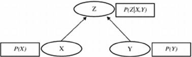
The quantitative expression comprises
probabilities of the variables. The figure below shows
a Bayesian Network with three variables X, Y and Z.
Variables X and Y are parents for variable Z, which
indicates that Z is the dependent node. The
probability for Z is a conditional probability based on
the probabilities of X and Y.
The probabilities in a Bayesian Network are
simplified by the DAG structure of the BN, by
applying directional separation (d-separation) (Pearl,
1988) and a Markov property assumption (Jensen and
Nielsen, 2007; Johnson et al., 2010), so that the
probability distribution of any variable is solely
dependent on its parents. Thus, the probability
distribution in a BN with n nodes
(X
1
,…,X
n
) can be formulated as:
A Systematic Review of Analytical Management Techniques in Business Process Modelling for SMEs Beyond
What-if-Analysis and Towards a Framework for Integrating Them with BPM
103

where Pa(X
i
) is the set of the probability distributions
corresponding to the parents of node X
i
(Heckerman
et al., 1995; Johnson et al., 2010). For the above
figure the above equation can be written as
P(Z)=P(Z|X,Y)∗P(X)∗P(Y).
Bayesian Networks based modelling relevant to
BPM framework has been recently investigated,
although not in depth, and only in the field of
customer modelling for some specific applications
(Ashcroft M., 2012; Anderson et al., 2004;
Chakraborty S., et. al., 2016).
2.4 The Cognitive Maps Approach in
Modelling Analysis
Cognitive maps (Axelrod, 1976), (Eden, 1992) are a
collection of nodes linked by some arcs or edges. The
nodes represent concepts or variables relevant to a
given domain. The causal links between these
concepts are represented by the edges. The edges are
directed to show the direction of influence. Apart
from the direction, the other attribute of an edge is its
sign, which can be positive (a promoting effect) or
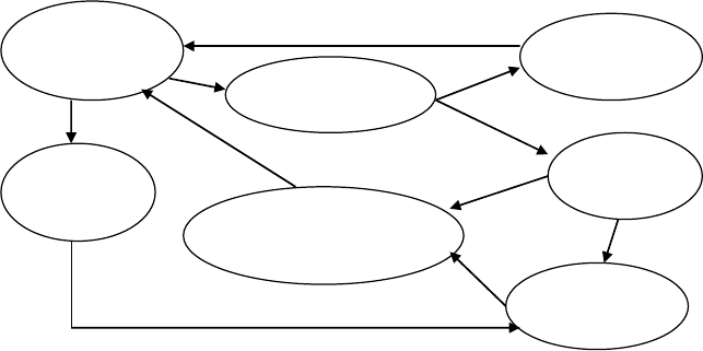
negative (an inhibitory effect). Cognitive maps can be
pictured as a form of signed directed graph. Figure 1
shows a cognitive map used to represent a scenario
involving some issues in public health.
BP1
BP2
BP3
BP4
BP6
BP5
BP7
+
+
+
+
+
+
+
-
-
-
Figure 1: Cognitive map concerning causal relations in
business processes within an enterprise.
The construction of a cognitive map requires the
involvement of a knowledge engineer and one or
more experts in a given problem domain. Methods for
constructing a cognitive map for a relatively recent
real-world application are discussed in (Tsadiras,
2003; Jetter, 2014).
The main objective of building a cognitive map
around a problem is to be able to predict the outcome
by letting the relevant issues interact with one
another. These predictions can be used for finding out
whether a decision made by someone is consistent
with the whole collection of stated causal assertions.
Such use of a cognitive map is based on the
assumption that, a person whose belief system is
accurately represented in a cognitive map, can be
expected to make predictions, decisions and
explanations that correspond to those generated from
the cognitive map. This leads to the significant
question: Is it possible to measure a person’s beliefs
accurately enough to build such a cognitive map? The
answer, according to Axelrod and his co-researchers,
is a positive one. Formal methods for analysing
cognitive maps have been proposed and different
methods for deriving cognitive maps have been tried
in (Axelrod, 1976).
In a cognitive map, the effect of a node A on another
node B, linked directly or indirectly to it, is given by
the number of negative edges forming the path
between the two nodes. The effect is positive if the
path has an even number of negative edges, and
negative otherwise. It is possible for more than one
such paths to exist. If the effects from these paths is a
mix of positive and negative influences, the map is
said to have an imbalance and the net effect of node
A on node B is indeterminate. This calls for the
assignment of some sort of weight to each inter-node
causal link, and a framework for evaluating combined
effects using these numerically weight-ed edges.
Fuzzy cognitive maps (FCM) (Caudill, 1990;
Brubaker, 1996a; Brubaker, 1996b) were proposed as
an extension of cognitive maps to provide such a
framework.
Fuzzy Cognitive Maps
The term Fuzzy Cognitive Map (FCM) was coined in
(Kosko, 1986) to describe a cognitive map model
with two significant characteristics:
(1) Causal relationships between nodes are fuzzified.
Instead of only using signs to indicate positive or
negative causality, a number is associated with the
relationship to express the degree of relationship
between two concepts.
(2) The system is dynamic involving feedback, where
the effect of change in a concept node affects
other nodes, which in turn can affect the node
initiating the change. The presence of feedback
adds a temporal aspect to the operation of the
FCM.
∏
=
=
n
i
iin
XPaXPXXXP
1
21
))(|(),...,,(
Seventh International Symposium on Business Modeling and Software Design
104

F-BP1
F-BP2
F-BP3
F-BP4
F-BP6
F-BP5
F-BP7
+0.1
+0.7
+0.9
+0.8
+0.9
+0.9
+0.6
-0.9
-0.3
-0.9
Figure 2: Fuzzified version of the cognitive map shown in Figure 1.
The FCM structure can be viewed as a recurrent
artificial neural network, where concepts are
represented by neurons and causal relationships by
weighted links or edges connecting the neurons.
By using Kosko’s conventions, the inter-
connection strength between two nodes C
i
and C
j
is
e
ij
, with e
ij
, taking on any value in the range -1 to 1.
Values –1 and 1 represent, respectively, full negative
and full positive causality, zero denotes no causal
effects and all other values correspond to different
fuzzy levels of causal effects. In general, an FCM is
described by a connection matrix E whose elements
are the connection strengths (or weights) e
ij
. The
element in the i
th
row and j
th
column of matrix E
represents the connection strength of the link directed
out of node C
i
and into C
j
. If the value of this link
takes on discrete values in the set {-1, 0, 1}, it is called
a simple FCM. The concept values of nodes C
1
, C
2
,
…, C
n
(where n is the number of concepts in the
problem domain) together represent the state vector
C.
An FCM state vector at any point in time gives a
snapshot of events (concepts) in the scenario being
modelled. In the example FCM shown in Figure 2,
node C
2
relates to the 2
nd
component of the state
vector and the state [0 1 0 0 0 0 0] indicates the event
"migration into city" has happened. To let the system
evolve, the state vector C is passed repeatedly
through the FCM connection matrix E. This involves
multiplying C by E, and then transforming the result
as follows:
C(k + 1) = T[C(k) . E]
where C(k) is the state vector of concepts at some
discrete time k, T is the thresholding or nonlinear
transformation function, and E is the FCM
connection matrix.
With a thresholding transformation function, the
FCM reaches either one of two states after a number
of passes. It settles down to a fixed pattern of node
values - the so-called hidden pattern or fixed-point
attractor. Alternatively, it keeps cycling between a
number of fixed states - known as the limit cycle.
With a continuous transformation function, a third
possibility known as the chaotic attractor (Elert,
1999) exists, when instead of stabilising, the FCM
continues to produce different state vector values for
each cycle.
Extensions of FCMs
A number of researchers have developed extended
versions of the FCM model described above. Tsadiras
(2003) and Jetter et al. (2014) describe the extended
FCM, in which concepts are augmented with memory
capabilities and decay mechanisms. The new
activation level of a node depends not only on the sum
of the weighted influences of other nodes but also on
the current activation of the node itself. A decay
factor in the interval [0,1] causes a fraction of the
current activation to be subtracted from itself at each
time step.
Park (1995) introduces the FTCM (Fuzzy Time
Cognitive Map), which allows a time delay before a
node x
i
has an effect on node x
j
connected to it
through a causal link. The time lags can be expressed
in fuzzy relative terms such as “immediate”,
“normal” and “long” by a domain expert. These terms
can be assigned numerical values such as 1, 2, 3. If
the time lag on a causal link e
ij
is m (1≥m) delay units,
then m – 1 dummy nodes are introduced between
node i and node j.
Decision-makers often find it difficult to cope
with significant real-world systems. These systems
are usually characterised by a number of concepts or
facts interrelated in complex ways. They are often
A Systematic Review of Analytical Management Techniques in Business Process Modelling for SMEs Beyond
What-if-Analysis and Towards a Framework for Integrating Them with BPM
105

dynamic ie, they evolve through a series of
interactions among related concepts. Feedback plays
a prominent role among them by propagating causal
influences in complicated pathways. Formulating a
quantitative mathematical model for such a system
may be difficult or impossible due to lack of
numerical data, its unstructured nature, and
dependence on imprecise verbal expressions. FCMs
provide a formal tool for representing and analysing
such systems with the goal of aiding decision making.
Given an FCM's edge matrix and an input
stimulus in the form of a state vector, each of the three
possible outcomes mentioned above can provide an
answer to a causal “what if” question. The inference
mechanism of FCMs works as follows. The node
activation values representing different concepts in a
problem domain are set based on the current state.
The FCM nodes are then allowed to interact
(implemented through the repeated matrix
multiplication mentioned above). This interaction
continues until:
(1) The FCM stabilises to a fixed state (the fixed-
point attractor), in which some of the concepts are
‘on’ and others are not.
(2) A limit cycle is reached.
(3) The FCM moves into a chaotic attractor state
instead of stabilising as in (1) and (2) above.
The usefulness of the three different types of
outcomes depends on the user’s objectives. A fixed-
point attractor can provide straightforward answers to
causal “what if” questions. The equilibrium state can
be used to predict the future state of the system being
modelled by the FCM for a particular initial state. As
an example based on figure 2, the state vector [0 1 0
0 0 0 0], provided as a stimulus to the FCM, may
cause it to equilibrate to the fixed-point attractor at [0
0 0 1 0 0 0]. Such an equilibrium state would indicate
that an increase in “migration into city” eventually
leads to the increase of “garbage per area”.
A limit cycle provides the user with a
deterministic behaviour of the real-life situation being
modelled. It allows the prediction of a cycle of events
that the system will find itself in, given an initial state
and a causal link (edge) matrix. For FCMs with
continuous transformation function and concept
values, a resulting chaotic attractor can assist in
simulation by feeding the simulation environment
with endless sets of events so that a realistic effect can
be obtained.
Development of FCMs for Decision Modelling
FCMs can be based on textual descriptions given by
an expert on a problem scenario or on interviews with
the expert. The steps followed are:
Step 1: Identification of key concepts/issues/factors
influencing the problem.
Step 2: Identification of causal relationships among
these concepts/issues/factors.
Experts give qualitative estimates of the strengths
associated with edges linking nodes. These estimates
are translated into numeric values in the range –1 to
1. For example, if an increase in the value of concept
A causes concept B to increase significantly (a strong
positive influence), a value of 0.8 may be associated
with the causal link leading from A to B. Experts
themselves may be asked to assign these numerical
values. The outcome of this exercise is a
diagrammatic representation of the FCM, which is
converted into the corresponding edge matrix.
Learning in FCMs
FCM learning involves updating the strengths of
causal links. Combining multiple FCMs is the
simplest form of learning. An alternative learning
strategy is to improve the FCM by fine-tuning its
initial causal link or edge strengths through training
similar to that in artificial neural networks. Both these
approaches are outlined below.
Multiple FCMs constructed by different experts
can be combined to form a new FCM. FCM
combination can provide the following advantages:
1. It allows the expansion of an FCM by
incorporating new knowledge embodied in other
FCMs.
2. It facilitates the construction of a relatively bias-
free FCM by merging different FCMs
representing belief systems of a number of experts
in the same problem domain.
The procedures for combining FCM are outlined in
(Kosko, 1988). Generally, combination of FCMs
involves summing the matrices that represent the
different FCMs. The matrices are augmented to
ensure conformity in addition. Each FCM drawn by
different experts may be assigned a credibility
weight. The combined FCM is given by:
k=N
∑ W
k
E
k
k=1
E =
where E is the edge matrix of the new combined
FCM, Ek is the edge matrix of FCM k, Wk is the
credibility weight assigned to FCM k, and N is the
number of FCMs to be combined. Siegel and Taber
Seventh International Symposium on Business Modeling and Software Design
106

(1987) outlines procedures for credibility weights
assignment in FCMs.
McNeill and Thro (1994) discuss the training of
FCMs for prediction. A list of state vectors is supplied
as historical data. An initial FCM is constructed with
arbitrary weight values. It is then trained to make
predictions of future average value in a stock market
using historical stock data. The FCM runs through the
historical data set one state at a time. For each input
state, the ‘error’ is determined by comparing the
FCM's output with the expected output provided in
the historical data. Weights are adjusted when error is
identified. The data set is cycled until the error has
been reduced sufficiently for no more changes in
weights to occur.
If a correlated change between two concepts is
observed, then a causal relation between the two is
likely and the strength of this relationship should
depend on the rate of the correlated change. This
proposition forms the basis of the Differential
Hebbian Learning (DHL). Kosko (1992) discusses
the use of DHL as a form of unsupervised learning for
FCMs. DHL can simplify the construction of FCMs
by allowing the expert to enter approximate values (or
even just the signs) for causal link strengths. DHL can
then be used to encode some training data to improve
the FCM’s representation of the problem domain and
consequently its performance.
Business Models as Cognitive Maps
Drawing on the insights of the cognitive mapping
approach in strategic management, we argue that the
causal structures embedded in business models can be
usefully conceptualized and represented as cognitive
maps (Furnari S., 2015). From this perspective, a
business model’s cognitive map is a graphical
representation of an entrepreneur or top manager’s
beliefs about the causal relationships inherent in that
business model (Furnari S., 2015). By emphasizing
the causal nature of business models, this definition is
consistent with previous studies viewing business
models as sets of choices and the consequences of
those choices (e.g. Casadesus-Masanell & Ricart,
2010), and with studies that explicitly highlight the
importance of cause-effect relationships in business
models’ cognitive representations (e.g. Baden-Fuller
& Haefliger, 2013; Baden-Fuller & Mangematin,
2013). Business models’ cognitive maps can be
derived from the texts that entrepreneurs and top
managers use in designing their business models, or
to pitch their projects to various audiences (including
investors, customers, policy makers); or they can be
derived from primary interviews with entrepreneurs
and top managers (Furnari S., 2015). Thus, the
content of a business model’s cognitive map can be
idiosyncratic, depending on the particular
individual’s cognitive schemas and on the language
they use. The raw concepts that entrepreneurs and top
managers use in their causal statements identify the
elements of a business model’s cognitive map that are
induced empirically (Furnari S., 2015). At the same
time, such maps may include elements deduced
theoretically from extant theories about business
models - i.e. the conceptual categories developed in
such theories (such as “value proposition”,
“monetization mechanisms”) - that can be useful to
classify the raw concepts used by entrepreneurs and
top managers, providing a basis for comparing
different individuals’ cognitive maps Thus, business
models’ cognitive maps include both inductive and
deductive elements, as do other types of cognitive
maps (e.g. Axelrod, 1976; Bryson et al., 2004)
For the sake of illustrating examples of business
models’ cognitive maps, we focus particularly on the
business model representation developed by Baden-
Fuller and Mangematin (2013), (Furnari S., 2015).
Among the several business model representations
suggested in the literature, we adopt this typological
representation because it strikes a balance between
parsimony and generality, thus meeting the criteria
typically recommended for solid theory-based
typologies (e.g. Doty & Glick, 1994; Delbridge &
Fiss, 2013). Specifically, this typology includes the
essential building blocks of the business model as
covered by other business model representations, thus
having a general scope in terms of content. At the
same time, it uses a more parsimonious set of
categories than other business model representations
in covering this general scope. For this reason, in the
cognitive maps’ illustrations provided below, we used
the four constructs characterizing this business model
representation (“customer identification”, “customer
engagement (or value proposition)”, “value chain”
and “monetization”) as organizing categories
(Furnari S., 2015). Although we use this specific
business model representation here for illustrating
business models’ cognitive maps, the cognitive
mapping approach developed in this paper can be
used, more generally, with any other business model
representation, depending on the analyst’s
preferences and research objectives (Furnari S.,
2015).
3 CONCLUSIONS
In this study we have attempted to present and analyse
some important analytical management techniques
A Systematic Review of Analytical Management Techniques in Business Process Modelling for SMEs Beyond
What-if-Analysis and Towards a Framework for Integrating Them with BPM
107

that are of value especially for SME, but through
extensions, under research, to larger scale enterprises
too. We have argued through examples relevant to
Business Process Modelling that in order for these
techniques to be widely utilized by enterprises a
common well defined framework should be
established based on BPM. BPM could provide the
representation schemes that should be integrated in
the associated formalisms. To this end, our
presentation is a first step. Each analytical
management technique herein presented should be
analysed in depth in order to be integrated with BPM
methodology in a common useful and well organized
application framework that in the sequel could be
employed in real world scenarios, managing even big
data of the associated enterprises.
REFERENCES
Ashcroft M. (2012), Bayesian networks in business
analytics, [in:] M. Ganzha, L. Maciaszek, M. Paprzycki
(Eds.), Proceedings of the Federated Conference on
Computer Science and Information Systems FedCSIS
2012, Polskie Towarzystwo Informatyczne, IEEE
Computer Society Press, Warsaw, Los Alamitos, CA
2012, pp. 955–961.
Anderson RD, Mackoy RD, Thompson VB, Harrell G.
(2004), A Bayesian network estimation of the service-
profit chain for transport service satisfaction. Decis Sci.
2004;35(4):665–89.
Axelrod R.M. (Ed.).(1976). Structure of decision: The
cognitive maps of political elites. Princeton: Princeton
University press.
Baden-Fuller C. & Morgan M. (2010). Business Models as
Models, Long Range Planning, 43(23): 156171
Baden-Fuller C. & Haefliger S. (2013). Business models
and technological innovation, Long Range Planning,
46(6): 419-426.
Baden-Fuller C., & Mangematin V. (2013). Business
models: A challenging agenda, Strategic Organization,
11(4), 418-427.
Barr P.S., Stimpert J.L. & Huff A.S. (1992). Cognitive
change, strategic action, and organizational renewal.
Strategic management journal, 13(S1): 15-36.
Bhargava, H. K., Herrick, C., Sridhar, S. (1999) “Beyond
Spreadsheets: Tools for Building Decision Support
Systems”, IEEE Expert, 32(3), 1999.
Brubaker, D. (1996a) "Fuzzy Cognitive Maps", EDN
Access, April 11 1996, [WWW document].
URL http://www.ednmag.com
Brubaker, D. (1996b) "More on Fuzzy Cognitive Maps",
EDN Access, April 25 1996b, [WWW document]. URL
http://www.ednmag.com
Bryson J.M., Ackermann F., Eden C. & Finn, C.B. (2004).
Visible thinking: Unlocking causal mapping for
practical business results, John Wiley & Sons.
Calori R., Johnson G. & Sarnin P. (1994). CEOs’ cognitive
maps and the scope of the organization, Strategic
Management Journal, 15: 437-457.
Carley K. & Palmquist M. (1992). Extracting, representing,
and analyzing mental models. Social forces, 70(3): 601-
636.
Casadesus-Masanell R. & Ricart J.E. (2010). From Strategy
to Business Models and onto Tactics. Long Range
Planning, 43(2-3): 195–215.
Caudill, M. (1990) “Using Neural Nets: Fuzzy Cognitive
Maps”, AI Expert, June 1990, pp. 49-53.
Chakraborty S., et. al. (2016), A Bayesian Network-based
customer satisfaction model: a tool for management
decisions in railway transport, Decision Analytics,
2016, 3:4,DOI: 10.1186/s40165-016-0021-2,
published:9/2016
Chesbrough H. & Rosenbloom R.S. (2002). The role of the
business model in capturing value from innovation:
Evidence from Xerox Corporation‘s technology spin-
off companies. Industrial and Corporate Change,
11(3): 529-555.
Chong, A., Khan, S., Gedeon, T. (1999a) “Differential
Hebbian Learning in Fuzzy Cognitive Maps: A
Methodological View in the Decision Support
Perspective”, Proc. Third Australia-Japan Joint
Workshop on Intelligent and Evolutionary Systems, 23-
25 Nov. 1999, Canberra (to be published).
Chong, A. (1999b) "Development of a Fuzzy Cognitive
Map Based Decision Support Systems Generator",
Honours dissertation, School of Information
Technology, Murdoch University, 1999.
Clarke, I., & Mackaness, W. (2001). Management
‘intuition’: an interpretative account of structure and
content of decision schemas using cognitive maps.
Journal of Management Studies, 38(2): 147-172.
Daly R, Shen Q, Aitken S. (2011), Learning Bayesian
networks: approaches and issues. Knowl Eng Rev.
2011;26(02):99–157.
Davis G.F. & Marquis C. (2005). Prospects for organization
theory in the early twenty-first century: Institutional
fields and mechanisms. Organization Science, 16(4):
332-343.
Delbridge R. & Fiss P.C. (2013). Editors' comments: styles
of theorizing and the social organization of knowledge.
Academy of Management Review, 38(3): 325-331.
Doganova L. & Eyquem-Renault M. (2009). What do
business models do?: Innovation devices in technology
entrepreneurship. Research Policy, 38(10): 1559–1570.
Doty D.H. & Glick W.H. (1994). Typologies as a unique
form of theory building: Toward improved
understanding and modeling. Academy of management
review, 19(2): 230-251.
Doz Y.L. & Kosonen M. (2010). Embedding Strategic
Agility: A Leadership Agenda for Accelerating
Business Model Renewal. Long Range Planning, 43(2–
3): 370–382.
Eden C., Ackermann F. & Cropper S. (1992). The analysis
of cause maps. Journal of Management Studies, 29(3):
309-324.
Seventh International Symposium on Business Modeling and Software Design
108

Eisenmann T., Parker G. & Van Alstyne M.W. (2006).
Strategies for two-sided markets. Harvard business
review, 84(10): 92.
Elert, G. (1999) The Chaos Hypertexbook, 1999,
http://hypertextbook.com/chaos/about.shtml
Elster J. (1998). A plea for mechanisms. in Hedström, P., &
Swedberg, R. (Eds.). Social mechanisms: An analytical
approach to social theory. Cambridge University Press.
Fiol C.M. & Huff A.S. (1992). Maps for managers: where
are we? Where do we go from here? Journal of
Management Studies, 29(3): 267-285.
Fox, T. (2005), Small and Medium-sized Enterprises
(SMEs) and Corporate Social Responsibility – A
Discussion Paper, International Institute for
Environment and Development, London.
Furnari, S. (2015), A Cognitive Mapping Approach to
Business Models: Representing Causal Structures and
Mechanisms, Chapter 8 in Business Models and
Modelling; Volume 33; Advances in Strategic
Management editors C. Baden-Fuller and V.
Mangematin; Emerald Press, 2015
Gavetti G.M., Henderson R. & Giorgi S. (2005) Kodak and
The Digital Revolution (A). Harvard Business School
Case #705-448.
Goldman I. (2012) ‘Poor decisions that humbled the Kodak
giant’. Financial Times. 13 April.
Grandori A. & Furnari S. (2008), A chemistry of
organization: Combinatory analysis and design,
Organization Studies, 29(2): 315-341.
Gunn R. and Williams W. (2007), Strategic tools: an
empirical investigation into strategy in practice in the
UK, Strat. Change 16: 201–216 (2007), Published
online in Wiley InterScience
(www.interscience.wiley.com) DOI: 10.1002/jsc.799
Heckerman D, Geiger D, Chickering DM. (1995), Learning
Bayesian networks: the combination of knowledge and
statistical data. Mach Learn. 1995;20:197–243
Hempel, C. G. (1965) ‘Fundamentals of Taxonomy, and
Typological Methods in the Natural and Social
Sciences’, Aspects of Scientific Explanation, ch. 6., pp.
137–72. New York: Macmillan.
Hodgkinson G.P., Bown N.J., Maule A.J., Glaister K.W. &
Pearman A.D. (1999). Breaking the frame: An analysis
of strategic cognition and decision making under
uncertainty, Strategic Management Journal, 20: 977-
985.
Hodgkinson G.P. & Healey M.P. (2008). Cognition in
organizations, Annual Review of Psychology, 59: 387-
417.
Hodgkinson G.P., Maule A.J. & Bown, N.J. (2004). Causal
cognitive mapping in the organizational strategy field:
A comparison of alternative elicitation procedures,
Organizational Research Methods, 7(1): 3-26.
Huff A.S. (1990). Mapping strategic thought. Chichester,
UK: Wiley.
Huff A.S., Narapareddy V. & Fletcher K.E. (1990). Coding
the causal association of concepts in Huff, A.S.
Mapping strategic thought, New York: John Wiley and
Sons.
Jenkins M. & Johnson G. (1997). Entrepreneurial intentions
and outcomes: A comparative causal mapping study.
Journal of Management Studies, 34: 895-920.
Jensen FV, Nielsen TD. (2007), Bayesian networks and
decision graphs. 2nd ed. Berlin: Springer; 2007
Jeppesen, S., Kothuis, B. and Tran, A.N. (2012), Corporate
Social Responsibility and Competitiveness for SMEs in
Developing Countries: South Africa and Vietnam,
Focales 16, Agence Francaise de Development, Paris.
Jetter Antonie J. and Kok K. (2014), Fuzzy Cognitive Maps
for futures studies—A methodological assessment of
concepts and methods, Futures journal, Volume 61,
September 2014, Pages 45–57, Elsevier,
https://doi.org/10.1016/j.futures.2014.05.002
Johnson S, Fielding F, Hamilton G, Mengersen K. (2010),
An integrated Bayesian network approach to lyngbya
majuscula bloom initiation. Mar Environ Res.
2010;69(1):27–37.
Kaplan S. & Sawhney M. (2000). B2B E-Commerce hubs:
towards a taxonomy of business models. Harvard
Business Review, 79(3): 97-100.
Kardaras, D., and Karakostas, B. (1999) "The use of Fuzzy
Cognitive Maps to Simulate Information Systems
Strategic Planning Process", Information and Software
Technology, Vol.41, Issue 4, 1999, pp. 197-210.
Klang D., Wallnöfer M. & Hacklin F. (2014). The Business
Model Paradox: A Systematic Review and Exploration
of Antecedents, International Journal of Management
Reviews.
Kosko, B. (1986) "Fuzzy Cognitive Maps", Int. J. Man-
Machine Studies, Vol.24, 1986, pp.65-75.
Kosko, B. (1992) “Neural Networks and Fuzzy Systems”,
Prentice Hall, Englewood Cliffs, NJ, 1992.
Lee, K.C., Kim, H. S. (1997) “A Fuzzy Cognitive Map-
based Bi-directional Inference Mechanism: An
Application to Stock Investment Analysis”, Intelligent
Systems in Accounting, Finance & Management, 6,
1997, pp. 41-57.
Lee, K.C., Lee, W.J., Kwon, O.B., Han, J.H., Yu, P.I.
(1998) “Strategic Planning Simulation Based on Fuzzy
Cognitive Map Knowledge and Differential Game",
Simulation, Nov. 1998, pp. 316-327.
Laukkanen M. (1994). Comparative cause mapping of
organizational cognitions, Organization science, 5(3):
322-343.
Luetkenhorst, W. (2004), “Corporate social responsibility
and the development agenda”,Intereconomics, Vol. 39
No. 3, pp. 157-166.
McNeill, M. F., and Thro, E. (1994) "Fuzzy Logic: A
Practical Approach", AP Professional Boston 1994.
Morsing, M. & Perrini, F., 2009. CSR in SMEs: do SMEs
matter for the CSR agenda?. Business Ethics: A
European Review, 18(1).
Nadkarni S, Shenoy PP. (2001) A Bayesian network
approach to making inferences in causal maps. Eur J
Oper Res. 2001;128(3):479–98.
Nadkarni S, Shenoy PP. (2004) A causal mapping approach
to constructing Bayesian networks. Dec Support Syst.
2004;38(2):259–81.
A Systematic Review of Analytical Management Techniques in Business Process Modelling for SMEs Beyond
What-if-Analysis and Towards a Framework for Integrating Them with BPM
109

Park, K.S. (1995) “Fuzzy Cognitive Maps Considering
Time Relationships”, International Journal of Human-
Computer Studies, Feb 1995, pp. 157-167.
Pearl J. (1988) Probabilistic reasoning in intelligent
systems. San Francisco: Morgan Kaufmann Publishers
Inc; 1988.
Power, D.J. (1997) "What is DSS?" DS*, The On-Line
Executive Journal for Data-Intensive Decision Support,
Vol.1, No.3, October 21, 1997, [WWW document].
URL: http://dss.cba.uni.edu/ papers/whatisadss
Rappa, M. A. (2004) ‘The Utility Business Model and the
Future of Computing Services’, IBM Systems Journal
43(1) 32–42.
Raynard, P. and Forstater, M. (2002), “Corporate social
responsibility: implications for small and medium
enterprises in developing countries”, UNIDO, Geneva,
available at: www.unido.org/fileadmin/import
/29959_CSR.pdf (accessed 27 September 2016).
Render, B., and Stair, M.S. (1988) "Quantitative Analysis
for Management", Allyn & Bacon, Boston 1988.
Salini S, Kenett RS. (2009), Bayesian networks of customer
satisfaction survey data. J Appl Stat.
2009;36(11):1177–89
Taber, R. (1991) “Knowledge Processing with Fuzzy
Cognitive Maps”, Expert Systems With Applications,
Vol. 2, 1991, pp. 83-87.
Tsadiras, Athanasios K. "Using fuzzy cognitive maps for e-
commerce strategic planning." Proc. 9th Panhellenic
Conf. on Informatics (EPY’2003). 2003.
Turban, E. (1993) Decision Support and Expert Systems
Management Support Systems, 3rd ed., Macmillan,
New York 1993.
VidHya Analytics (2017), Introduction to Markov chain :
simplified!,
(https://www.analyticsvidhya.com/blog/2014/07/mark
ov-chain-simplified/) accessed 1/2017
Wirtz, B. W., Schilke, O. and Ullrich, S. (2010) ‘Strategic
Development of Business Models: Implications of the
Web 2.0 for Creating Value on the Internet’, Long
Range Planning 43(2–3): 272–90.
Seventh International Symposium on Business Modeling and Software Design
110